The standard error of the mean describes how much a sample mean varies across repeated samples under a specified sampling model. For independent, identically distributed observations with finite variance, its population value is \(\frac{\sigma}{\sqrt{n}}\).
Because the population standard deviation σ is usually unknown, a common estimate replaces it with the sample standard deviation s: \(\text{estimated SEM}=\frac{s}{\sqrt{n}}\). This estimates uncertainty in a mean, rather than variation among individual observations.
Calculate SEM from a sample
Use the observations 1 3 5. Their mean is 3. The squared deviations from 3 are 4, 0, and 4, giving a total of 8. Divide by \(n-1=2\) to get the sample variance, 4. Its square root gives \(s=2\).
Now divide by \(\sqrt{3}\): \(\text{estimated SEM}=\frac{2}{\sqrt{3}}\approx1.1547\). The mean, sample SD, and SEM all use the same units as the original observations. The variance uses squared units.
If a sample already has a reported SD of 10 units and \(n=25\), the calculation is \(\frac{10}{5}=2\) units. Check that the reported number really is an SD, rather than an SEM or a confidence-interval half-width.
Why independence matters
For independent observations with the same finite variance \(\sigma^{2}\), the variance of their mean is \(\frac{\sigma^{2}}{n}\). Taking the square root gives \(\frac{\sigma}{\sqrt{n}}\). Correlation introduces additional covariance terms, so the shortcut can be inappropriate for repeated, clustered, or time-dependent data.
Complex surveys, sampling a substantial part of a finite population without replacement, and unequal weighting may need design-specific standard errors. A raw row count does not by itself establish the amount of independent information.
SD and SEM answer different questions
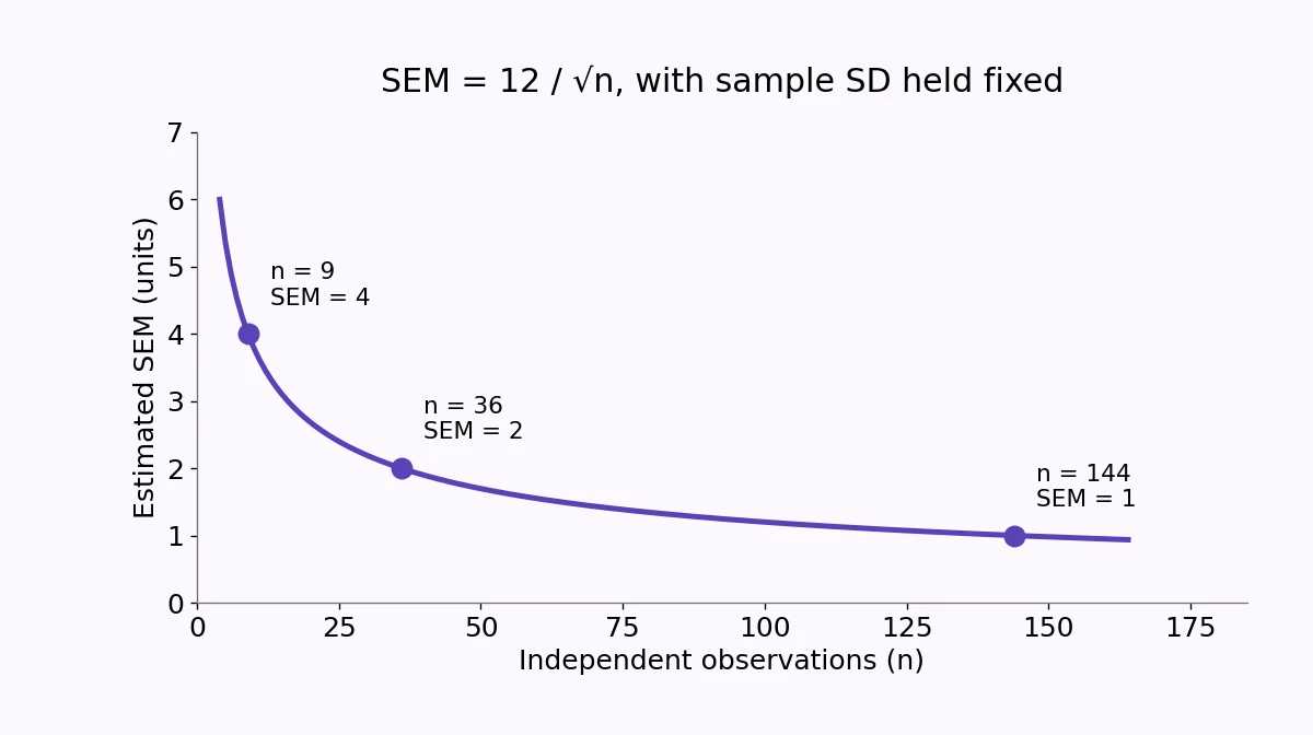
SD describes the spread of observations. SEM describes uncertainty in an estimated mean. Keeping s fixed while increasing n reduces estimated SEM, but does not reduce the spread of the individual observations in that calculation.
For \(s=12\), \(n=9\) gives \(\operatorname{SEM}=4\); \(n=36\) gives \(\operatorname{SEM}=2\). Four times the sample size halves the SEM. In real data, s can also change as observations are collected.
SEM is not a confidence interval
A two-sided interval needs a multiplier and assumptions. For an independent normal sample with unknown σ, a confidence interval for the mean uses the Student t distribution with \(n-1\) degrees of freedom: \(\text{mean}\pm t\times\frac{s}{\sqrt{n}}\).
Putting one SEM on either side of a mean does not create a 95% confidence interval. Label SD, SEM, and interval bars explicitly and include the sample size and method.
Small samples and missing values
Estimating s with the usual \(n-1\) divisor requires at least two observations. A very small sample can give an unstable estimate of variability. Normality is not required for the variance identity under the independence assumptions, but it matters for an exact small-sample t interval.
Decide how missing observations are handled and report the actual count used. Silently mixing a sample SD computed from one group with the count from another changes the result.