Linear functions are a visual representation of values that create a straight line. By using the proper equation to graph a line values can be represented over time. These values can then be used to find more information and solve problems. Linear programming is the process of graphing sets of data together to find maximal and minimal benefits.
This kind of solution could be used in a business to calculate the optimal amount of investment versus optimal productivity to provide optimal profit. Inversely, the same information could be used to find minimal productivity to show profits.
Graphing Inequalities
The purpose of linear programming is to provide a visual basis for inequalities. These inequalities are graphed to optimize input and output.
When linear functions are graphed the data can be shown as a visual representation of either input or output. However, variations in the data are subject to criteria that cannot be displayed through linear functions. This means a different kind of problem solving is needed.
Graphing linear functions can display known data and can also be used to show inequalities that provide contrast to known variables. This is called a linear relationship. The equations used to maximize, find variations, and optimize are deceptively simple.
Mathematical Optimization
These three equations have very distinct functions, but they use the same data. The equation to maximize uses c to represent known vectors of coefficients and x to represent variable vectors of coefficients. The function of ( . ) T is used to flip the matrix diagonally to make it more easily represented on the graph.
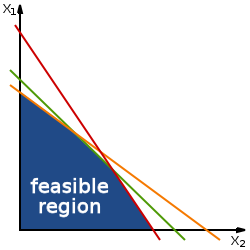
Inequalities, or constraints, are represented in Ax ≤ b and x ≥ 0. The combination of the maximize and subject to functions form the feasible region, or the area in which input or output must fall in to optimize for the known data.
Examples of Optimization
If a farmer needs to plant two kinds of crops and make a profit, he will need to calculate the cost of fertilizer per square kilometer, the cost of pesticide per square kilometer, and the selling price of both crops. The variable in the problem will need to be represented as F for fertilizer, P for pesticide, S for selling price, and L for land. Increments of these variables will be represented by square kilometers.
Each kilometer, or x, of one crop requires F1 and P1. The second type of crop will require F2 and P2 per x2.
The first step is to maximize the revenue with the equation of, S1 * x1 + S2 * x2 = Revenue. Next the constraints will need to be calculated. x1 + x2 < L represents the limit of total area available to plant in. F1 * x1 + F2 * x2 < F represents the limit of fertilizer, or F. P1 * x1 + P2 * x2 < P will represent the limit of pesticide. Finally, x1 > 0, x2 > 0 represents the constraint that crops can’t be planted in a negative area.
This information can be used to form a matrix which can then be used to calculate the revenue generated by selling the crops. With this algorithm, the farmer will be able to predict profits and costs, allowing him to optimize efforts in order to make enough money by the end of the season.