Conditional formatting can highlight duplicates while leaving every record in place. That makes it useful for reviewing customer IDs, invoice numbers, or repeated entries before deciding whether anything should be removed. A matching ID is a reason to inspect a record, not proof that the entire row is redundant.
We will highlight repeated customer IDs, extend the highlight across complete rows, and show an alternative that flags only occurrences after the first. The example deliberately includes a blank ID and two records that share an ID but have different statuses.
Paste the example records
Paste the tab-separated block below into a blank sheet at A1 to enter these fictional records. The records occupy A2:D8. Keep the first cell of the Trial row empty: that blank is part of the example, not a missing instruction.
| Row | A | B | C | D |
|---|---|---|---|---|
| 1 | Customer ID | Name | Status | |
| 2 | C101 | Maya | maya@example.test | Paid |
| 3 | C102 | Omar | omar@example.test | Pending |
| 4 | C103 | Lin | lin@example.test | Paid |
| 5 | C101 | Maya | maya@example.test | Paid |
| 6 | C104 | Ana | ana@example.test | Paid |
| 7 | Trial | trial@example.test | Pending | |
| 8 | C102 | Omar | omar@example.test | Paid |
Copy the tab-separated data below into A1. The worksheet letters and row numbers above are display labels, not part of the data.
Customer ID	Name	Email	Status
C101	Maya	maya@example.test	Paid
C102	Omar	omar@example.test	Pending
C103	Lin	lin@example.test	Paid
C101	Maya	maya@example.test	Paid
C104	Ana	ana@example.test	Paid
	Trial	trial@example.test	Pending
C102	Omar	omar@example.test	Paid
C101 appears in sheet rows 2 and 5; C102 appears in rows 3 and 8. We want those four rows flagged. C103 and C104 each occur once. Row 7 has no customer ID, so we will exclude it from the rule.
Highlight repeated values in one column
- Select
A2:A8, without the header. - Open Format → Conditional formatting.
- Under Format cells if, choose Custom formula is.
- Enter the formula below, choose a fill color, and click Done.
=AND(A2<>"",COUNTIF($A$2:$A$8,A2)>1)COUNTIF counts how often the current ID appears in the complete list. A count greater than one identifies a repeated value. The A2<>"" test excludes blank IDs. AND requires both tests to be true before the formatting is applied.
The dollar signs lock the counting range to A2:A8. The final A2 remains relative, so Sheets checks A3 on the next row, then A4, and so on. The reference must start on the same row as the selected range; using A1 here would shift the test away from its record.
Highlight the entire matching row
For a table that is easier to review, change the rule’s application range to A2:D8 and use this version:
=AND($A2<>"",COUNTIF($A$2:$A$8,$A2)>1)The $A reference fixes the ID column while the row number can change. Without that column lock, cells farther across a row could test the name, email, or status instead of the customer ID. The expected highlighted rows are still 2, 3, 5, and 8.
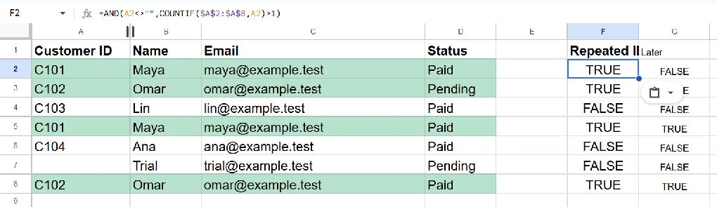
Notice that the two C102 records are not identical: one says Pending and the other says Paid. The rule identifies the repeated key, not an exact duplicate across all four columns. You might need to reconcile a payment update rather than discard a row. Review the business meaning before deleting anything.
Flag only the second and later occurrences
If you want the first occurrence to stay unmarked, replace the whole-row rule with:
=AND($A2<>"",COUNTIF($A$2:$A2,$A2)>1)The counting range now grows from row 2 to the current row. The first C101 has appeared once at that point; the second has appeared twice. The same reasoning applies to C102. Only sheet rows 5 and 8 should be highlighted. This identifies later occurrences in the current row order, so sorting the records can change which occurrence is considered first.
Avoid misleading matches
COUNTIF text matching is not case-sensitive, so this rule does not distinguish an ID written as C101 from c101. If letter case is meaningful in your identifiers, you need a case-sensitive method. Leading or trailing spaces can also make apparently similar IDs behave differently; examine and clean a copy before relying on the highlight.
These steps describe the desktop browser interface. Menu placement can differ in mobile apps. The formulas use English names and comma separators; a semicolon locale may require different argument separators. After adding new records, extend both the formatting range and the fixed counting range. Keep a visible legend or explain the rule to anyone reviewing the sheet, so color is not the only clue to its meaning.
For other ways to organize and check records, visit our Google Sheets tutorials.