Use FILTER to return rows that satisfy several conditions in Google Sheets. You can build a separate list of open support tickets, unpaid invoices, or orders from a particular region without moving or deleting the source records. Changing a condition updates the result produced by the formula.
Our fictional ticket table includes two teams, two priorities, and two statuses. We will start with open Support tickets, add a priority test, and then distinguish AND logic from an either/or condition.
Prepare a source table and an output area
Paste the tab-separated source block below at A1 in a blank sheet. The headers occupy A1:E1, and the records occupy A2:E8. Leave columns G through K empty below row 3: the filtered output needs room to expand across five columns.
| Row | A | B | C | D | E |
|---|---|---|---|---|---|
| 1 | Ticket | Team | Priority | Status | Hours |
| 2 | T01 | Support | High | Open | 3 |
| 3 | T02 | Sales | High | Open | 2 |
| 4 | T03 | Support | Low | Closed | 1 |
| 5 | T04 | Support | High | Closed | 4 |
| 6 | T05 | Support | High | Open | 2 |
| 7 | T06 | Sales | Low | Open | 1 |
| 8 | T07 | Support | Low | Open | 5 |
Copy the tab-separated data below into A1. The worksheet letters and row numbers above are display labels, not part of the data.
Ticket	Team	Priority	Status	Hours
T01	Support	High	Open	3
T02	Sales	High	Open	2
T03	Support	Low	Closed	1
T04	Support	High	Closed	4
T05	Support	High	Open	2
T06	Sales	Low	Open	1
T07	Support	Low	Open	5
The first question is simple: which tickets belong to Support and are still Open? Reading the table gives T01, T05, and T07. Those ticket IDs give us a small independent check before relying on the formula.
Apply two conditions
Enter this formula in G4:
=FILTER(A2:E8,B2:B8="Support",D2:D8="Open")A2:E8 is the complete range to return. The region of the formula after it contains two tests: the team must equal Support, and the status must equal Open. Each condition describes the same seven source rows. A ticket is included only when both tests are true for that ticket.
The result should fill G4:K6 with these three records, in their original order:
| Row | G | H | I | J | K |
|---|---|---|---|---|---|
| 4 | T01 | Support | High | Open | 3 |
| 5 | T05 | Support | High | Open | 2 |
| 6 | T07 | Support | Low | Open | 5 |
These are the expected values without worksheet labels. Use them for comparison; keep the formula in the output area.
T01	Support	High	Open	3
T05	Support	High	Open	2
T07	Support	Low	Open	5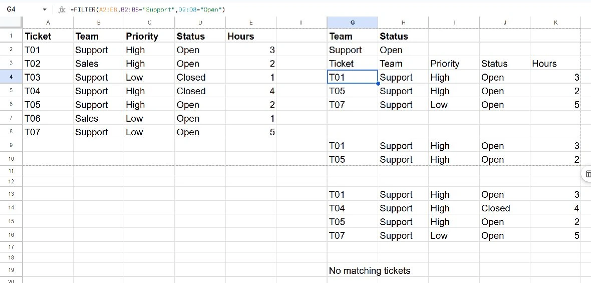
T04 belongs to Support but is Closed, so it is left out. T02 is Open but belongs to Sales, so it is also left out. FILTER returns the records themselves; it does not add the Hours column or create a summary total.
Use cells as report controls
Put Team in G1 and Status in H1. Enter Support in G2 and Open in H2. You can now replace the formula in G4 with:
=FILTER(A2:E8,B2:B8=G2,D2:D8=H2)The output remains the same, but you can change the question by editing the two control cells. For example, choosing Sales and Open returns T02 and T06. Do not place the controls inside the area where the formula expands: input cells and output cells need separate space.
To keep only High-priority tickets for the chosen team and status, replace the formula with:
=FILTER(A2:E8,B2:B8=G2,D2:D8=H2,C2:C8="High")With Support and Open still selected, this returns T01 and T05. Adding a separate condition argument adds another required test; it does not widen the list to include either condition.
Combine an either/or test with a required condition
Suppose the team must be Support, while the ticket can be either High priority or Open. Use:
=FILTER(A2:E8,B2:B8="Support",(C2:C8="High")+(D2:D8="Open"))The addition combines the two parenthesized logical tests as an OR condition. The separate team test still applies to every result. This version returns T01, T04, T05, and T07. T04 qualifies through its priority even though it is closed; T07 qualifies through its status even though its priority is low.
Handle empty results and range errors
When no rows match, FILTER returns #N/A. For example, this dataset has no Support tickets with a Waiting status. If an empty report is an expected outcome, use:
=IFNA(FILTER(A2:E8,B2:B8="Support",D2:D8="Waiting"),"No matching tickets")The result is No matching tickets. IFNA handles a no-match error rather than concealing every possible problem. An underlying #N/A error can also trigger the message, so inspect source errors if a report looks unexpectedly empty.
If the output cannot expand because cells already contain data, clear or move those cells instead of deleting source records. Keep all condition ranges the same height as the data range. Extend every range together when you add records; a formula ending at row 8 will not automatically include row 9.
Examples use English function names and comma argument separators. Some locales require semicolons between arguments. Keep the comparison labels unchanged, check the expected ticket IDs, and use our Google Sheets tutorials for related workflows.