Use SUMIFS to add amounts only when every condition is satisfied. It is useful when a total needs to match a region, payment status, sales channel, or another combination of fields. You can ask for paid orders from the East without counting pending orders or sales from another region.
This example uses a small fictional order list. First, we calculate a total with two conditions. Then we move the conditions into cells and add a third test, keeping the original records intact.
Set up an order list
Use the tab-separated data block below to enter this example in a blank sheet at A1. The headers should occupy A1:E1, with seven orders in rows 2 through 8. Enter the amounts as numbers, without typing a currency symbol into the value itself; you can apply currency formatting afterward.
| Row | A | B | C | D | E |
|---|---|---|---|---|---|
| 1 | Order | Region | Channel | Status | Amount |
| 2 | O101 | East | Online | Paid | 120 |
| 3 | O102 | West | Online | Paid | 80 |
| 4 | O103 | East | Online | Pending | 90 |
| 5 | O104 | East | Store | Paid | 150 |
| 6 | O105 | East | Online | Paid | 110 |
| 7 | O106 | West | Store | Pending | 60 |
| 8 | O107 | East | Store | Paid | 70 |
Copy the tab-separated data below into A1. The worksheet letters and row numbers above are display labels, not part of the data.
Order	Region	Channel	Status	Amount
O101	East	Online	Paid	120
O102	West	Online	Paid	80
O103	East	Online	Pending	90
O104	East	Store	Paid	150
O105	East	Online	Paid	110
O106	West	Store	Pending	60
O107	East	Store	Paid	70
Our question is: What is the total amount for East orders with a Paid status? Four orders qualify: O101, O104, O105, and O107. Their amounts are 120, 150, 110, and 70, so the expected total is 450.
Add two conditions with SUMIFS
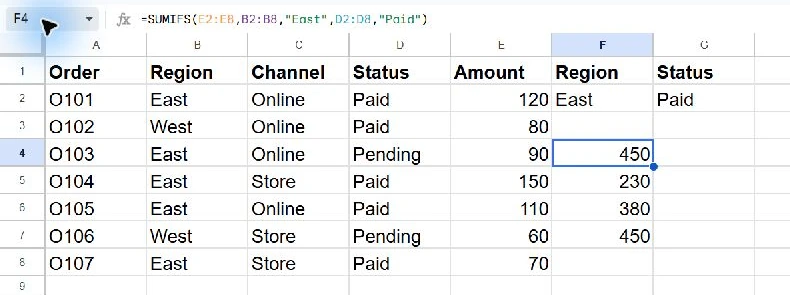
Click an empty cell, such as F4, and enter:
=SUMIFS(E2:E8,B2:B8,"East",D2:D8,"Paid")The first argument, E2:E8, contains the numbers to add. The next pair checks the region in B2:B8 against "East". The final pair checks the status in D2:D8 against "Paid". All three ranges describe the same seven orders.
Each row is evaluated as one record. O103 has the right region but the wrong status, so its amount of 90 is excluded. O102 is paid but belongs to the West, so its 80 is also excluded. The function does not combine a matching region from one row with a matching status from another.
Put your criteria in cells
For a report you will reuse, put Region in F1 and Status in G1. Enter East in F2 and Paid in G2. Replace the formula in F4 with:
=SUMIFS(E2:E8,B2:B8,F2,D2:D8,G2)The result remains 450. Change F2 to West, and the same formula returns 80. This separates the question from the calculation: a reader can change the controls without editing the formula. Cell references do not need quotation marks; fixed text criteria do.
Add another condition
Return F2 to East. To include only East orders that are both paid and online, enter this formula in another empty cell, such as F5:
=SUMIFS(E2:E8,B2:B8,F2,D2:D8,G2,C2:C8,"Online")Only O101 and O105 qualify, giving 120 + 110 = 230. To find paid East orders worth at least 100, use a numeric comparison instead:
=SUMIFS(E2:E8,B2:B8,"East",D2:D8,"Paid",E2:E8,">=100")Enter that formula in F6. It includes 120, 150, and 110, giving 380. The comparison operator belongs inside the quoted criterion. If a threshold lives in another cell, join it to the operator, for example ">="&H2.
Check a surprising total
Multiple criteria use AND logic. Asking for East and West in two criteria pairs on the same region column does not mean either region; one order cannot equal both labels. For an either/or question, use a method designed for that logic rather than adding an incompatible test.
If a result is zero unexpectedly, inspect the data before changing the function. Check for trailing spaces in labels, amounts stored as text, and ranges that start or end on different rows. Keep headers outside the numeric range. When adding orders below row 8, extend every participating range together so the report includes them.
These examples use English function names and commas between arguments. A sheet using semicolons as argument separators needs semicolons in those positions; do not change punctuation inside a quoted criterion. Compare the four qualifying orders with the total before applying the pattern to a larger report.
Explore more practical data tasks in our Google Sheets tutorials.