Use SUMIFS to add amounts only when every condition on the same row is satisfied. For example, you can total online revenue from the East region without adding store sales or another region’s orders.
This walkthrough uses a small, hypothetical sales ledger. You will build one formula, check the matching rows by hand, and then turn the criteria into cells you can change. The examples use English function names and comma separators; some regional Excel settings require semicolons.
1. Paste the example sales data
Copy the tab-separated block below into cell A1 of a blank worksheet. The headers belong in row 1, and the six records occupy rows 2 through 7. Amounts are in dollars; the negative amount is a refund.
Region	Channel	Amount
East	Online	120
West	Online	200
East	Store	150
East	Online	80
East	Online	-20
West	Store	90
Columns A and B describe each transaction. Column C contains the numbers to add. Keep these columns aligned: a condition in row 5 must select the amount from row 5, not the next row.
2. Add East-region online revenue
Enter this formula in E2:
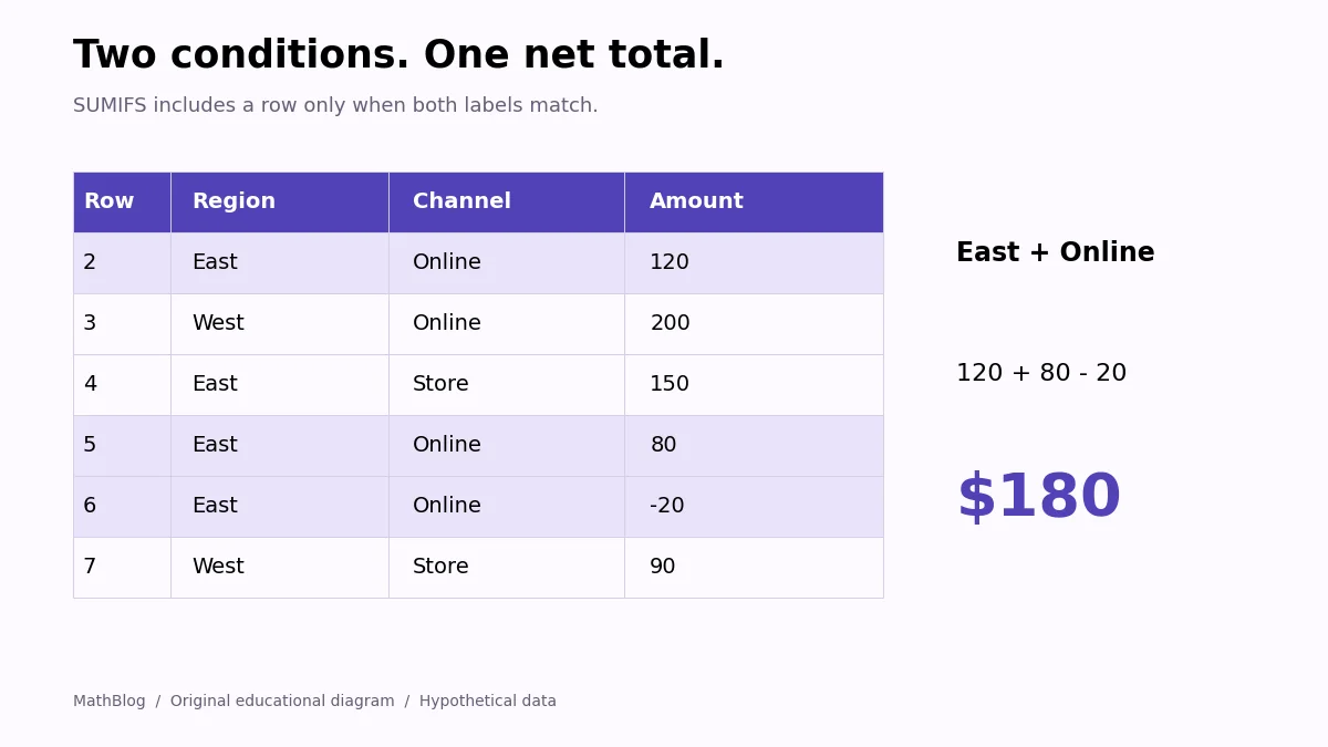
=SUMIFS(C2:C7,A2:A7,"East",B2:B7,"Online")The result is 180. The qualifying amounts are 120, 80, and -20, so the independent check is 120 + 80 - 20 = 180. The 150 store sale does not qualify, even though it is in the East region.
Read the arguments from left to right: start with the amount range, then give a criteria range and its condition. Repeat those last two arguments for each additional condition. SUMIFS combines the conditions with AND, meaning each included record must pass all of them.
3. Put the conditions in editable cells
Enter Region in F2 and East in G2. Enter Channel in F3 and Online in G3. Replace the formula in E2 with:
=SUMIFS($C$2:$C$7,$A$2:$A$7,G2,$B$2:$B$7,G3)It still returns 180. Change G2 to West, and it returns 200; change G3 to Store, and it returns 90. Cell references are not surrounded by quotation marks. The dollar signs keep the source ranges fixed if you copy this formula elsewhere.
This small criteria area is useful for a reusable report. Someone can choose a different region without editing the calculation itself, and the selected conditions remain visible beside the answer.
4. Add a numeric condition deliberately
To add only positive East online amounts, add the amount column as another criteria range:
=SUMIFS(C2:C7,A2:A7,"East",B2:B7,"Online",C2:C7,">0")This returns 200, because it leaves out the -20 refund. That is a different question from net revenue. Keep the refund in the original 180 total when you want the signed value of all qualifying transactions.
For a threshold stored in G4, use ">"&G4 as the criterion. The comparison operator stays in quotes; the ampersand attaches the cell’s value.
When you mean OR rather than AND
A row cannot have both Online and Store in its Channel cell. For West sales through either channel, add two separate totals:
=SUMIFS(C2:C7,A2:A7,"West",B2:B7,"Online")+SUMIFS(C2:C7,A2:A7,"West",B2:B7,"Store")The result is 290. This addition is safe here because the channel labels do not overlap. If your two rules can both match the same row, simply adding their totals can count that amount twice.
Check an unexpected result
- Use equal-sized ranges. Every range here begins at row 2 and ends at row 7.
- Check the data type. Amounts imported as text may not contribute as intended. Test a suspect cell with
=ISNUMBER(C2). - Inspect labels. An extra trailing space can make a category fail to match the intended label.
- Do not assume filters change the calculation. SUMIFS still evaluates matching rows hidden by an ordinary worksheet filter.
- Include new records. If you append row 8, extend every relevant range together; a formula ending at row 7 cannot include it.
For more practical spreadsheet workflows, visit the MathBlog Excel tutorials. Start by deciding precisely which records belong in your total, then make the formula express that rule.