A running total adds each new value to everything above it. In Excel, an expanding SUM range gives you the cumulative amount on every row, so you can see progress toward a target rather than just one final total.
We will use seven hypothetical daily sales figures, then show how the same idea handles a starting balance or a refund. The basic method uses ordinary cell formulas and does not require a PivotTable or a newer dynamic-array function.
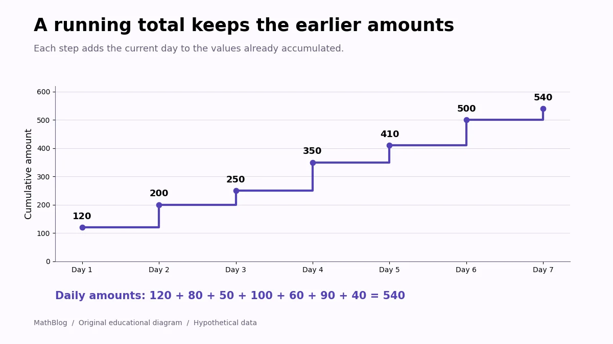
1. Set up the daily amounts
Paste this tab-separated block into A1. The header belongs in row 1, with amounts in B2:B8. Day 1 through Day 7 are labels for an already ordered sequence, not actual calendar dates.
Day	Amount
Day 1	120
Day 2	80
Day 3	50
Day 4	100
Day 5	60
Day 6	90
Day 7	40
Type Running total in C1. Each result in column C will answer “How much has accumulated through this row?” Keep the input amounts in column B separate from the calculated totals.
2. Enter an expanding SUM formula
In C2, enter:
=SUM($B$2:B2)The first result is 120, because the range currently includes only B2. Copy C2 down through C8, using the fill handle or your usual copy-and-paste method.
The starting reference, $B$2, stays fixed. The ending reference, B2, moves as you copy down. In C3, Excel therefore sums B2:B3; in C4 it sums B2:B4.
| Cell | Formula | Expected result |
|---|---|---|
| C2 | =SUM($B$2:B2) | 120 |
| C3 | =SUM($B$2:B3) | 200 |
| C4 | =SUM($B$2:B4) | 250 |
| C5 | =SUM($B$2:B5) | 350 |
| C6 | =SUM($B$2:B6) | 410 |
| C7 | =SUM($B$2:B7) | 500 |
| C8 | =SUM($B$2:B8) | 540 |
A quick independent check is 120 + 80 + 50 + 100 + 60 + 90 + 40 = 540. That should match the last cumulative result, not the sum of the cumulative results.
3. Keep an opening balance separate
If you begin with 250 already accumulated, type Opening balance in E2 and 250 in F2. Replace the formula in C2 with:
=$F$2+SUM($B$2:B2)Copy it down to C8. The first result becomes 370, and the last becomes 790. F2 is fixed so every row starts from the same opening amount. Do not enter the opening balance as an extra sale as well, or you will add it twice.
When amounts can raise or lower a starting balance, the output is often called a running balance. The formula still works; the meaning depends on what the input values represent.
4. Allow refunds to reduce the total
Return C2 to the original formula without the opening balance, and copy down. Now change B5, the Day 4 amount, from 100 to -30. This example replaces that day’s value with a refund rather than adding a separate transaction.
The results become 120, 200, 250, 220, 280, 370, and 410. A running sum does not have to increase on every row. If a negative transaction is legitimate, the decrease is useful information rather than a formula error.
Order and range checks that matter
- Sort complete records together. A running total depends on order. In a real dated ledger, sort the whole table by the intended transaction date and any tie-breaking identifier.
- Do not freeze both ends.
=SUM($B$2:$B$2)copied down repeats the first amount. - Do not move both ends.
=SUM(B2:B2)copied down returns each individual amount. - Check new rows. Append the next amount and copy the formula into that row. A blank calculation cell will not create its own running result.
- Do not add column C to report total sales. Earlier transactions appear repeatedly in it. Sum the original amounts in B instead.
A cumulative total also does not reset automatically for a new customer or month. For this basic formula, the starting row defines the beginning of one sequence. Choose a separate grouped method when each category needs its own accumulation.
Continue with the Excel tutorials on MathBlog when you need another way to summarize or organize the original records.