XLOOKUP finds an ID in one range and returns the corresponding value from another range. In Google Sheets, you can make the match exact and supply a clear message for IDs that are not present.
We will look up product prices in a small fictional catalog. The example deliberately includes an unsorted list and a repeated ID, because finding a result is only useful when you understand which record supplied it.
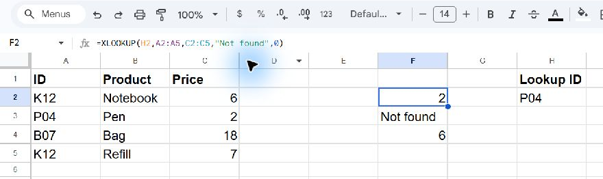
Paste the product catalog
Copy this tab-separated block into A1 on a blank worksheet:
| Row | A | B | C |
|---|---|---|---|
| 1 | ID | Product | Price |
| 2 | K12 | Notebook | 6 |
| 3 | P04 | Pen | 2 |
| 4 | B07 | Bag | 18 |
| 5 | K12 | Refill | 7 |
Copy only the tab-separated block below. Worksheet letters and row numbers in the preview are display labels, not part of the data.
ID	Product	Price
K12	Notebook	6
P04	Pen	2
B07	Bag	18
K12	Refill	7
The lookup IDs are in A2:A5; the prices are in C2:C5. Product descriptions in column B help you inspect the selected row. K12 appears twice on purpose: once for a notebook and once for a refill. A production catalog should normally give different products different unique identifiers.
Next, set up the lookup input:
Copy this tab-separated block into H1 on a blank worksheet:
| Row | H |
|---|---|
| 1 | Lookup ID |
| 2 | P04 |
Copy only the tab-separated block below. Worksheet letters and row numbers in the preview are display labels, not part of the data.
Lookup ID
P04
H2 now contains P04. Leave F2:F4 available for the three calculations below. These formulas use English names and comma separators; adjust separators if your sheet locale requires it.
Return the price for the selected ID
Enter this formula in F2:
=XLOOKUP(H2,A2:A5,C2:C5,"Not found",0)The expected result is 2, the price in C3 for P04. XLOOKUP searches A2:A5 for the value in H2, then returns the value at the corresponding position in C2:C5.
The final 0 explicitly requests an exact match. We do not want a nearby product ID when the requested product is missing. The list does not have to be sorted for this ordinary first-to-last exact search.
Change H2 to B07. F2 should become 18. Restore H2 to P04 before comparing the original example again. Keeping the input in a separate cell lets you reuse the calculation without rewriting the lookup formula.
Give missing IDs a useful label
In F3, test an ID that does not exist:
=XLOOKUP("Z99",A2:A5,C2:C5,"Not found",0)The result is Not found. That is a missing match, not a price of zero. Returning zero for an absent product could make an incomplete catalog look as though it contained a free item.
The missing-value argument handles the absent match. It is preferable to wrapping the entire calculation in a broad error replacement when you only intend to label missing IDs. A wrongly sized result range, for example, deserves investigation.
Understand what a duplicate ID does
Enter this in F4:
=XLOOKUP("K12",A2:A5,C2:C5,"Not found",0)The expected result is 6, from the first K12 record, not 7 from the second. The default search direction begins at the first entry and works downward. XLOOKUP returns a match; it does not certify that the key is unique.
If duplicate IDs represent multiple valid transactions, decide whether you actually need all records or a grouped total. Choosing the first record is usually the wrong substitute for such a summary. If they represent inconsistent master data, repair that problem before using the price in an order calculation.
Keep lookup and result ranges aligned
A2:A5 and C2:C5 start and end on the same rows. Changing the second range to C3:C6 would shift every returned value, even though it has the same number of cells. Alignment matters as much as matching range lengths.
Inspect imported IDs for text-versus-number differences and extra spaces. Preserve leading zeros when they belong to an identifier, and avoid converting catalog keys to numbers just to make a match work. Add new products to both referenced ranges, or revise the range strategy deliberately.
Before using a larger catalog, test one known ID, one absent ID, and one duplicated ID. Those three checks reveal whether your formula’s match policy agrees with the meaning of the source data.