Continuity corrections are used in statistics to improve the approximation of a discrete probability distribution with a continuous distribution. This correction is necessary because discrete distributions (typically binomial distributions) deal with distinct, countable outcomes, whereas continuous distributions (usually the normal distribution) describe probabilities over a continuous range.
When analyzing data that is discrete, such as counts or frequencies, it is often necessary to make statistical inferences assuming a continuous distribution. This assumption can lead to inaccuracies in the calculations, particularly when dealing with small sample sizes or extreme values. To address this issue, the continuity correction introduces an adjustment factor.
What Is the Continuity Correction Factor?
When using continuity correction, you adjust the discrete value by a small amount (usually 0.5) to better align with the continuous framework. For example, if you are calculating the probability of observing up to a certain number of successes in a binomial distribution, you would adjust this number by adding or subtracting 0.5, and then use this adjusted value in the corresponding continuous distribution’s formula.
This adjustment helps in mitigating the error that arises from directly substituting a discrete distribution with a continuous one, making the approximation more accurate.
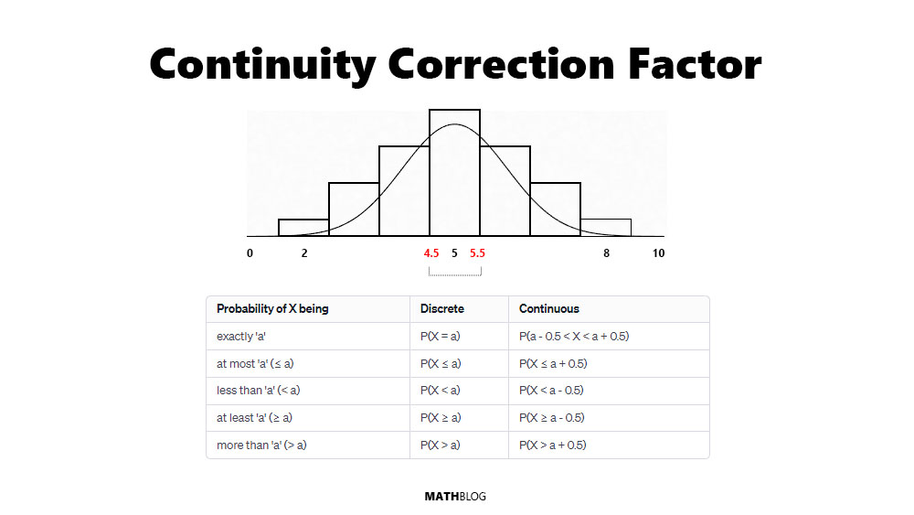
Use the table below to know when to add or to substract a continuity correction factor:
| Probability of X being | Discrete | Continuous |
|---|---|---|
| exactly ‘a’ | P(X = a) | P(a – 0.5 < X < a + 0.5) |
| at most ‘a’ (≤ a) | P(X ≤ a) | P(X ≤ a + 0.5) |
| less than ‘a’ (< a) | P(X < a) | P(X < a – 0.5) |
| at least ‘a’ (≥ a) | P(X ≥ a) | P(X ≥ a – 0.5) |
| more than ‘a’ (> a) | P(X > a) | P(X > a + 0.5) |
According to the central limit theorem the continuity correction should only be applied when both \( n \times p \) (the expected number of successes) or \( n \times (1 – p) \) (the expected number of failures) are equal to or greater than 5. When these values are both at least 5, it typically indicates that the sample size \( n \) is large enough for the normal approximation to be valid.
Check out our continuity correction calculator for ease of computation.
Discrete vs. Continuous Distributions
To appreciate the essence of continuity correction, it’s essential to first understand the distinction between discrete and continuous distributions. Discrete distributions, like the binomial or Poisson distributions, deal with countable outcomes. In contrast, continuous distributions, such as the normal distribution, involve data that can take on any value within a range. The transition from a discrete to a continuous framework, while often convenient, isn’t straightforward and necessitates adjustments – this is where the continuity correction factor comes into play.
Continuity Correction and Z-scores
Once continuity correction is applied, the next step is to calculate the Z-score. The Z-score, also known as a standard score, is a statistical measurement that describes a value’s relationship to the mean of a group of values, measured in terms of standard deviations from the mean. It’s a way of standardizing scores on a common scale.
The formula for calculating a Z-score in a dataset is:
\( Z = \frac {(X – \mu)}{\sigma} \)

The Z-score transformation is essential for a few reasons:
- Standardization: Z-scores standardize different data points, allowing them to be compared and analyzed on a common scale. This is crucial in approximations where we are transitioning from a specific discrete distribution to the standard normal distribution.
- Ease of Probability Calculation: The standard normal distribution (a normal distribution with a mean of 0 and a standard deviation of 1) is well-tabulated and widely used. By converting our corrected value to a Z-score, we can easily look up the probability associated with this score in standard normal distribution tables or calculate it using statistical software.
- Statistical Inference: Z-scores are fundamental in statistical hypothesis testing and confidence interval estimation. In the context of approximating discrete distributions, calculating the Z-score allows us to use the extensive tools and methods developed for normal distributions, including hypothesis tests and confidence intervals.
- Accuracy in Approximation: The calculation of Z-scores, combined with Continuity Correction, results in a more accurate approximation of probabilities. This is especially important in cases where precise probability estimation is critical, such as in medical trials, quality control processes, and risk assessment models.
Related: Try our Z-score calculator.
Continuity Correction in Practice
Let’s consider a practical example. Suppose you’re approximating a binomial distribution with \( n = 40 \) and \( p = 0.3 \) using a normal distribution. Calculate the probability of getting at most 10 successes in our binomial example above using continuity correction.
Solution
The given values are:
- Number of trials (n): \( n = 40 \)
- Probability of success (p): \( p = 0.3 \)
- Number of successes we are interested in (k): \( k = 10 \)
STEP 1: Is the sample size large enough?
Because \( 40 \times 0.3 = 12 \) and \( 40 \times (1 – 0.3) = 28 \), both are greater than 5 so the continuity correction factor can be used.
STEP 2: Calculate the Mean and Standard Deviation
Mean: \( \mu = n \times p = 40 \times 0.3 = 12 \)
Standard Deviation: \( \sigma = \sqrt{n \times p \times (1 – p)} = \sqrt{40 \times 0.3 \times (1 – 0.3)} = \sqrt{8.4} \approx2.8982 \)
STEP 3 : Apply Continuity Correction
The problem says “at most 10 successes”, that means P(X ≤ 10) so we need to +0.5 based on our table above. That means we need to find P(X < 10.5).
Adjusted value of X: \( X_{corrected} = 10 + 0.5 = 10.5 \)
STEP 4: Calculate the Z-score
\( Z = \frac{X_{corrected} – \mu}{\sigma} \approx \frac{10.5−12}{2.8982} \approx−0.5175 \)
Quick note:
- A Z-score of 0 indicates that the data point is exactly at the mean.
- A positive Z-score indicates that the data point is above the mean.
- A negative Z-score indicates that the data point is below the mean.
STEP 5: Find the Corresponding Probability
The probability corresponding to a Z-score of -0.5175, according to the standard normal distribution (check the Z-table) is \( \approx 0.3024 \). This means that there’s a 30.24% chance of observing at most 10 successes with continuity correction.