About 50,000 people read my article 3 awesome free Math programs. Chances are that at least some of them downloaded and installed Maxima. If you are one of them but are not acquainted with CAS (Computer Algebra System) software, Maxima may appear very complicated and difficult to use, even for the resolution of simple high school or calculus problems. This doesn’t have to be the case though, whether you are looking for more math resources to use in your career or a student in an online bachelor’s degree in math looking for homework help, Maxima is very friendly and this 10 minute tutorial will get you started right away. Once you’ve got the first steps down, you can always look up the specific function that you need, or learn more from Maxima’s official manual. Alternatively, you can use the question mark followed by a string to obtain in-line documentation (e.g. ? integrate). This tutorial takes a practical approach, where simple examples are given to show you how to compute common tasks. Of course this is just the tip of the iceberg. Maxima is so much more than this, but scratching even just the surface should be enough to get you going. In the end you are only investing 10 minutes.
Maxima as a calculator
You can use Maxima as a fast and reliable calculator whose precision is arbitrary within the limits of your PC’s hardware. Maxima expects you to enter one or more commands and expressions separated by a semicolon character (;), just like you would do in many programming languages.
(%i1) 9+7;
(%o1) [tex]16[/tex]
(%i2) -17*19;
(%o2) [tex]-323[/tex]
(%i3) 10/2;
(%o3) [tex]5[/tex]
Maxima allows you to refer to the latest result through the % character, and to any previous input or output by its respective prompted %i (input) or %o (output). For example:
(%i4) % - 10;
(%o4) [tex]-5[/tex]
(%i5) %o1 * 3;
(%o5) [tex]48[/tex]
For the sake of simplicity, from now on we will omit the numbered input and output prompts produced by Maxima’s console, and indicate the output with a => sign. When the numerator and denominator are both integers, a reduced fraction or an integer value is returned. These can be evaluated in floating point by using the float function (or bfloat for big floating point numbers):
8/2;
=> [tex]4[/tex]
8/2.0;
=> [tex]4.0[/tex]
2/6;
=> [tex]\displaystyle \frac{1}{3}[/tex]
float(1/3);
=> [tex]0.33333333333333[/tex]
1/3.0;
=> [tex]0.33333333333333[/tex]
26/4;
=> [tex]\displaystyle \frac{13}{2}[/tex]
float(26/4);
=> [tex]6.5[/tex]
As mentioned above, big numbers are not an issue:
13^26;
=> [tex]91733330193268616658399616009[/tex]
13.0^26
=> [tex]\displaystyle 9.1733330193268623\text{ }10^_{+28}[/tex]
30!;
=> [tex]265252859812191058636308480000000[/tex]
float((7/3)^35);
=> [tex]\displaystyle 7.5715969098311943\text{ }10^_{+12}[/tex]
Constants and common functions
Here is a list of common constants in Maxima, which you should be aware of:
- %e – Euler’s Number
- %pi – [tex]\displaystyle \pi[/tex]
- %phi – the golden mean ([tex]\displaystyle \frac{1+\sqrt{5}}{2}[/tex])
- %i – the imaginary unit ([tex]\displaystyle \sqrt{-1}[/tex])
- inf – real positive infinity ([tex]\infty[/tex])
- minf – real minus infinity ([tex]-\infty[/tex])
- infinity – complex infinity
We can use some of these along with common functions:
sin(%pi/2) + cos(%pi/3);
=> [tex]\displaystyle \frac{3}{2}[/tex]
tan(%pi/3) * cot(%pi/3);
=> [tex]1[/tex]
float(sec(%pi/3) + csc(%pi/3));
=> [tex]3.154700538379252[/tex]
sqrt(81);
=> [tex]9[/tex]
log(%e);
=> [tex]1[/tex]
Defining functions and variables
Variables can be assigned through a colon ‘:’ and functions through ‘:=’. The following code shows how to use them:
a:7; b:8;
=> [tex]7[/tex]
=> [tex]8[/tex]
sqrt(a^2+b^2);
=> [tex]\sqrt{113}[/tex]
f(x):= x^2 -x + 1;
=> [tex]x^2 -x + 1[/tex]
f(3);
=> [tex]7[/tex]
f(a);
=> [tex]43[/tex]
f(b);
=> [tex]57[/tex]
Please note that Maxima only offers the natural logarithm function log. log10 is not available by default but you can define it yourself as shown below:
log10(x):= log(x)/log(10);
=> [tex]\displaystyle log10(x):=\frac{log(x)}{log(10)};[/tex]
log10(10)
=> [tex]1[/tex]
Symbolic Calculations
factor enables us to find the prime factorization of a number:
factor(30!);
=> [tex]\displaystyle 2^{26}\,3^{14}\,5^7\,7^4\,11^2\,13^2\,17\,19\,23\,29[/tex]
We can also factor polynomials:
factor(x^2 + x -6);
=> [tex](x-2)(x+3)[/tex]
And expand them:
expand((x+3)^4);
=> [tex]\displaystyle x^4+12\,x^3+54\,x^2+108\,x+81[/tex]
Simplify rational expressions:
ratsimp((x^2-1)/(x+1));
=> [tex]x-1[/tex]
And simplify trigonometric expressions:
trigsimp(2*cos(x)^2 + sin(x)^2);
=> [tex]\displaystyle \cos ^2x+1[/tex]
Similarly, we can expand trigonometric expressions:
trigexpand(sin(2*x)+cos(2*x));
=> [tex]\displaystyle -\sin ^2x+2\,\cos x\,\sin x+\cos ^2x[/tex]
Please note that Maxima won’t accept 2x as a product, it requires you to explicitly specify 2*x. If you wish to obtain the TeX representation of a given expression, you can use the tex function:
tex(%);
=> $$-\sin ^2x+2\,\cos x\,\sin x+\cos ^2x$$
Solving Equations and Systems
We can easily solve equations and systems of equations through the function solve:
solve(x^2-4,x);
=> [tex]\displaystyle \left[ x=-2 , x=2 \right][/tex]
%[2]
=> [tex]x=2[/tex]
solve(x^3=1,x);
=> [tex]\displaystyle \left[ x={{\sqrt{3}\,i-1}\over{2}} , x=-{{\sqrt{3}\,i+1}\over{2}}  , x=1 \right][/tex]
trigsimp(solve([cos(x)^2-x=2-sin(x)^2], [x]));
=> [tex]\displaystyle \left[ x=-1 \right][/tex]
solve([x - 2*y = 14,  x + 3*y = 9],[x,y]);
=> [tex]\left[ \left[ x=12 , y=-1 \right]  \right][/tex]
2D and 3D Plotting
Maxima enables us to plot 2D and 3D graphics, and even multiple functions in the same chart. The functions plot2d and plot3d are quite straightforward as you can see below. The second (and in the case of plot3d, the third) parameter, is just the range of values for x (and y) that define what portion of the chart gets plotted.
plot2d(x^2-x+3,[x,-10,10]);
plot2d([x^2, x^3, x^4 -x +1] ,[x,-10,10]);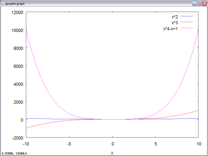
f(x,y):= sin(x) + cos(y);
plot3d(f(x,y), [x,-5,5], [y,-5,5]);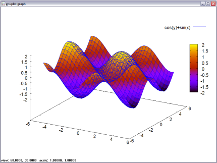
Limits
limit((1+1/x)^x,x,inf);
=> %[tex]e[/tex]
limit(sin(x)/x,x,0);
=> [tex]1[/tex]
limit(2*(x^2-4)/(x-2),x,2);
=> [tex]8[/tex]
limit(log(x),x,0,plus);
=> [tex]-\infty[/tex]
limit(sqrt(-x)/x,x,0,minus);
=> [tex]-\infty[/tex]
Differentiation
diff(sin(x), x);
=> [tex]\displaystyle cos(x)[/tex]
diff(x^x, x);
=> [tex]\displaystyle x^{x}\,\left(\log x+1\right)[/tex]
We can calculate higher order derivatives by passing the order as an optional number to the diff function:
diff(tan(x), x, 4);
=> [tex]\displaystyle 8\,\sec ^2x\,\tan ^3x+16\,\sec ^4x\,\tan x[/tex]
Integration
Maxima offers several types of integration. To symbolically solve indefinite integrals use integrate:
integrate(1/x, x);
=> [tex]\displaystyle log(x)[/tex]
For definite integration, just specify the limits of integrations as the two last parameters:
integrate(x+2/(x -3), x, 0,1);
=> [tex]\displaystyle -2\,\log 3+2\,\log 2+{{1}\over{2}}[/tex]
integrate(%e^(-x^2),x,minf,inf);
=> [tex]\sqrt{\% pi}[/tex]
If the function integrate is unable to calculate an integral, you can do a numerical approximation through one of the methods available (e.g. romberg):
romberg(cos(sin(x+1)), x, 0, 1);
=> 0.57591750059682
Sums and Products
sum and product are two functions for summation and product calculation. The simpsum option simplifies the sum whenever possible. Notice how the product can be use to define your own version of the factorial function as well.
sum(k, k, 1, n);
=> [tex]\displaystyle \sum_{k=1}^{n}{k}[/tex]
sum(k, k, 1, n), simpsum;
=> [tex]\displaystyle {{n^2+n}\over{2}}[/tex]
sum(1/k^4, k, 1, inf), simpsum;
=> [tex]\displaystyle {{\%pi^{4}}\over{90}}[/tex]
fact(n):=product(k, k, 1, n);
=> [tex]fact(n):=product(k,k,1,n)[/tex]
fact(10);
=>  [tex]3628800[/tex]
Series Expansions
Series expansions can be calculated through the taylor method (the last parameter specifies the depth), or through the method powerseries:
niceindices(powerseries(%e^x, x, 0));
=> [tex]\displaystyle \sum_{i=0}^{\infty }{{{x^{i}}\over{i!}}}[/tex]
taylor(%e^x, x, 0, 5);
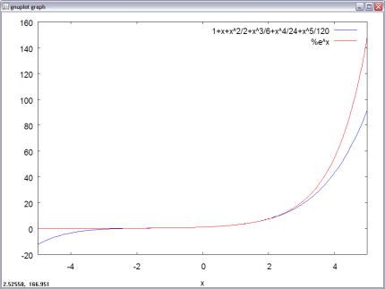
=> [tex]\displaystyle 1+x+{{x^2}\over{2}}+{{x^3}\over{6}}+{{x^4}\over{24}}+{{x^5}\over{120 }}+\cdots[/tex]
The trunc method along with plot2d is used when taylor’s output needs to be plotted (to deal with the [tex]+\cdots[/tex] in taylor’s output):
plot2d([trunc(%), %e^x], [x,-5,5]);
I hope you’ll find this useful and that it will help you get started with Maxima. CAS can be powerful tools and if you are willing to learn how to use them properly, you will soon discover that it was time well invested.
This is awesome. Awesome! Thank you.
— Josh
Cool beans. Very nice write-up.
nice infos, in my opinion these kind of software should be much more supported by universities, instead of (implicitly) encouraging the use of pirated software…
thanks! I was just trying to improve my Maxima skills…
ciao ciao!
Thank you. Very useful intro.
Wow. Looks awesome. The thing that REALLY sealed the deal was the TeX output. Love it.
Great software. Great for my high school subject.
this was NOT a guide for high school calc…
it’s a great, vague, manual snapshot
..
a guide would have a scan from a high school calc book, and STEPS with screenshots
man, where was all this cool free math software when I was stuck using maple on mac plus? argh!
probably a good thing that it “appears” difficult as it’d a shame for highschoolers to simply use it instead of learning basic algebra.
This is awesome little tool. Wish I knew about this in my school.
I have been using Maxima as I re-learn Algebra. I use it it verify what I do by hand, but sometimes I would like to see some of the intermediate steps. Is there any way to do that?
How the hell do you translate these formulas to be used in software programs like javascript and actionscript?
Could you possibly create a tutorial on what all the symbols mean?
Excellent write-up. How did you get the LaTeX output on the fly? The presentation looks great!
The fancy calculus stuff doesn’t translate. Most of the basic functions (sin, sqrt, log, etc) are available as Math.sin() and whatnot. Google for “javascript math” to get a full list of Javascript’s math functions and constants.
@rwinston
Thank you very much. I used a LaTeX plugin for Wordpress, and I wrote the TeX code for simple cases and Maxima’s tex(expr) function for the longer ones.
great job ! do u know of a similar tutorial for R ?
@easan
Thanks a lot easan. For R, take a look at this tutorial: https://www.cyclismo.org/tutorial/R/
This is really cool, sadly the school year is now over and I can’t use it!!! fdasdafhasdkj! GRRR!
Maxima has its roots in Macsyma which existed before Mathematica and Maple.
See the following article about Macsyma:
https://en.wikipedia.org/wiki/Macsyma
I’ve recommended Maxima to many people. Most of these people rejected it and did not even bother to look it up because they never heard of the name or believe free software cannot be of good quality.
I would like to see a side-to-side comparison between Maxima and the commercial alternatives. I can imagine Mathematica and Maple having more features (never missed them though) and a more optimized solver.
great program! helps a lot at the university
Thanks!
I’d messed with Maxima a few months ago, and found it a painful experience trying to figure it out from the manual. Went thru your tutorial last night and now I can use this for solving real problems.
This will be a HUGE asset for me.
Alex
Hi!The information was delivered in a simple way that it is very easy to understand in using the software which initially i found it very difficult to use Maxima when I explore it al by my own. But now you had help me to solve my probs.
It is indeed a fantastic piece of info for me especially at this moment in rushing my assignment. Thanks…
Got exactly what I wanted.
Thank you so much@
Hi
Thanks for the Tut. However I cant find information to help me. My problem is as follows:
I want to solve f in the following two functions, when I choose the following:
s=2400 and d = 2000. f is the required value, which is the focal point of a parabole.
h=d^2/(16*f);
s=d/2*(sqrt((4*h/d)^2+1))+2*f*ln((4*h/d)+sqrt((4*h/d)^2+1));
I substitude h in the second function and then evaluate for the said values of s and d.
All goes well and is calculated. However I then can not get a calculated value for f from Maxima. The following eauation is given.
2400=2*ln(500/f+sqrt(250000/f^2+1))*f+1000*sqrt(250000/f^2+1)
What can I do to get a calculated value for f?
Thanks
Jacobus
with Mathematica, I can do wonderful things to turn a series of calculations into a semi-professional looking document. Can I do that with maxima? (or wmaxima, or …?) I’ve played with it (on windows) and it just seems like a ‘calculator’ I can solve it all, but it’s not really made to give a nice formatted output. Seems. I claim no full knowledge, maybe I’m missing something.
Thank you. Your article is very useful to me to start with with Maxima.
Rajendra
JiK, you can use Maxima from within TeXmacs or from a SAGE notebook.
i think that knowing all this math will be very helpful in the long run. it should really help you in the future
Any suggestions on how to get Maxima to generate a surface of revolution; e.g., the surface formed between y=x^2, y=0 and x=6 is revolved about either axis?
Thanks.
Very usefull. Muito bom mesmo.
fantastic program! great work guys!
After a short tutorial, I tried a real problem:
solve([x*(1+(0.083/y)^(1/z))-41, x*(1+(0.833/y)^(1/z))-44.9, x*(1+(8.333/y)^(1/z))
-47.8], [x,y,z]);
____
But get no response, anything I was wrong?
Hr.stein, I run your system of equations and as a response I got that it has no solutions ([]).
thanks for your reply, Antonio!
In fact, I would expect an approximate solution using least square approach, with indication of deviation.( somewhat like the Mathematica does).
I still think Maxima could solve the equations, only I miss some built-in functions or there is mistake in my expression.
Regards!
log (3m+7)-log (m+4)= 2log 6 – 3log 3
6 6 6 6
This is a fantastic tutorial. Thanks to the author, I was able to discover the great power of this amazing program. Based on this page, I started to write a tutorial for Maxima in Greek.
https://lomik.wordpress.com/maxima/
Hello
How can I tell maxima that a given variable is real and greater than zero in the expression below?
integrate((a/pi)/(a^2+x^2),x,-inf,inf)
fantastic!! This is a great getting started tutorial and showes the power of the program.
I teach at University of Colorado and really push the value and quality of open source software (which I use in my own research). Next time I teach numerical analysis I will definitly use Maxima!
Excellent!! Thanks for your great tutorial for Maxima.
Wow, just from reading about the Maxima wants me to use it, it seems that its a very powerful mathematical tool
I used to lust after Mathematica but it is outrageously expensive: $2,500. We are approaching the point where open source alternatives, like Maxima, are the way to go for heavy duty computer assisted symbolic and numerical mathematics.
I like the way you are presenting this material. I have used Maxima and Scilab in teaching a course on Computation. I am a big fan of Maxima. Scilab is OK but crashes a lot. ON the other hand Maxima is extremely solid with many options for the user interface. It is promoted as a symbolic math program but it can do most of the run of the mill numerical math. Here is the link to the course material I taught.
https://www.eng.ysu.edu/~jalam/engr6924s07/
Feel free to take any part of the material if you want to write more articles about math calculation using Maxima.Also any feed back from is highly welcomed.
Very nice tutorial, Antonio. I’m signing up for your RSS feed.
Tell me, is there a way to zoom and rotate the 3d graphs? Also, my graphs are not solid planes like your screenshots but rather grids. How does one make the planes solid? Thanks.
Richard,
Use assume(a>0);
Dotan,
To make the graphs coloured and solid you could add [gnuplot_pm3d,true] to the end of the statement eg:
plot3d(f(x,y), [x,-5,5], [y,-5,5],[gnuplot_pm3d,true]);
Re: Jacobus
Better late than never?
(%i1) find_root(subst( [h=d^2/(16*f),d=2000,s=2400], s=d/2*(sqrt((4*h/d)^2+1))+2*f*log((4*h/d)+sqrt((4*h/d)^2+1))),f,1,2400);
(%o1) 421.811063853618
I’ve 2 issues here:
FIRST: Halting problem in TM
——
The below symbolic example doesn’t terminate after many minutes in maxima-5.14.0 although the human solution is f(x)-g(x)-h(x):
factor(expand((f(x)-g(x)-h(x))^500));
To fix this problem in the future: better
artificial sustitution in the solving of
factor or intelligent lazy computation as
factor(expand(Alpha)) => Alpha.
SECOND: Non-deterministic Memoization
——-
With
factor(expand((sqrt(x+a)+b)^10));
i got once the imprecise solution
10 b x^4 sqrt(x+a) + 120 b^3 x^3 sqrt(x+a) + … + 45 a^4 b^2 + a^5
but i got many times sqrt(x+a)+b)^10 .
I think that the maxima system
uses memoization that remember some
internal answers of previous computations
but it’s non-deterministic.
axima 5.14.0 (with CLISP 2.41) has 2 symbolic bugs:
* First bug: it doesn’t factor when it uses sqrt instead sqrt2 :
(%i1) factor(expand((sqrt(x)+y)^2));
2
(%o1) y + 2 sqrt(x) y + x
(%i2) factor(expand((sqrt2(x)+y)^2));
2
(%o2) (y + sqrt2(x))
* Second bug: wrong result due to the sign: (y-x)^1000 instead of (x-y)^1000 :
(%i3) factor(expand((x-y)^1000));
1000
(%o3) (y – x)
Is there any way to get nice looking latex fonts in the EuMathT notebook? For example, if one calculates >:integrate(x,x) one gets
x^2
—–
2
and this in not nice looking. How to get LaTeX fonts?
Seem like a good maths tool. Students of maths should welcome this tool. Nowadays, learners go for effective learning tools. This is a good target.
WOuld you know how to do this problem? I am extremely stuck!!! And confused!! The problem is Convert 400 ft/sec to mi/hr. I get how to convert the ft to mi but I am completely stuck on the sec to hr. I would really appreciate some help. 🙂
Sylvia, try to replace ft with the amount of miles in a foot, and sec with the amount of hours in a second.
1 ft = 1/5280 mi (a mile has 5280 feet)
1 sec = 1/3600 hr (an hour has 3600 seconds)
400 ft/sec = 400 * (1/5280 mi) / (1/3600 hr) = (400 * 3600)/5280 mi/hr = 272.72… mi/hr
As far as I remember, if you change the fonts in the main screen to Greek, you can also see the symbols like %pi displayed.
Great tutorial,
Thanks.
hi
can any one help me to solve this question
Given that U = {x : x is real numbers}, A = {x : x is positive integer}, B = {x : x is negative integers}, C = {x : x = , where a and b are integers with b 0}. Draw separate Venn diagrams for each of the following sets, shading those areas that represent the set.
(a) M = {1, 3, 5 ,7 ,9 …..}
(b) P = {x : x2 = 2}
(c) Q = {x : (2 – x) > 3, x is integers}
(d) R = {x : 2x = 0}
(e) T = {x : x = 2πr, r is a positive integers, π is Pi}
Sir,
Would you please give the format or code for solving the Fredholm Integral eqn.
g(r)= lambda*integral from 0 to infinity of
f(x)*K(x,r)dx
g(r) and K(x,r) being known.
I tried the function ieqn(ie, unk, tech, n, guess), but I am unable to supply the required parameters seperately. It will be helpfull if you could illustrate it with an example.
Thanks in advance
yeswanthl@sify.com
A very awesome tutorial,
make a lot of fun!
Thank You.
This guide is exactly what a beginner need to have a look to Maxima in 10 minutes. I would be happy to find it for any software.
I suggest you to add few lines in guide about GNU TeX macs and SAGE. It’s an important feature in my opinion, mainly for beginners, and I saw it only browsing the messages.
Thank you very much.
As the last comment was from ’07, just wanted to let you know your effort is still appreciated. About 2 days into this, and the main manual is terrible to learn from, even for syntax. Helped a little that I knew Lisp. Picked up a few new items from your examples.
Thanks.
Thanks for this great tutorial. I picked up enough in 10 minutes to know that Maxima is pretty awesome and worth learning well.
Great tutorial!! Thanks for your effort!!!
Now if there only were a proper commenting and (gnu)plot-export functionality like in Maple and Mathematica..it’d be also usable.
Nice idea ! Wonderful program ! Bye angelo
Thanks a lot!
skeeeeen man
I am amazed with the use of Maxima software. I am becoming familiar with it. It solves many problems.
It is difficult for me to understand many of the commands. I would like someone to help me in converting decimal numbers to binary numbers by using Maxima. Give me the commands used only.
Thank you.
Wow Man , Thank you for promoting open source software !
This is a great alternative to expensive commercial CAS, like Mathematica. In fact, I wish there were more tutorials of this sort, thanks!
It’s so useful, thank you so much. I going to check paciently¡
Best, Zxoch.m
Yeah, this tutorial is pretty awesome. As much as I like Maxima, it’s documentation sucks for high school and bachelor-level students… This is really great and needed… Maybe you should post a tutorial on how to program in Maxima — this will show it’s on par with mathematica…
Hi Antonio,
Many thanks for posting this, it saved me a lot of work (and in this case euros, because I didn’t need to buy a program 🙂 )!
Keep up the work and all the best,
Gijs
Nice summary.
Hi
i’m just wondering if maxima could solve numerical diferencial systems?
i’m looking for a tutorial, anyone can help me?
Very good.
Do you happen to know about any tutorial on optimization in maxima? (using numerical algorithms)
excellent maxima intro!
ny suggestions on how to get Maxima to generate a surface of revolution; e.g., the surface formed between y=x^2, y=0 and x=6 is revolved about either axis?
Thanks.
What ever I did with pricy mathematica, I can do with maxima+TeXmacs. Goodbye mathematica, hello maxima. Thanks Antonio
It is possible to generate plots of 3d vector fields with maxima?
Maxima may be powerful, and very useful to career mathematicians, but the interface is pretty poor. It’s not intuitive and not easy to discover how to use things. At the least, you should use WxMaxima as a front-end, which gives it a decent graphical interface with common functions in menus. Even this needs a lot more polish, though.
Noice! I love the free programs AND math
Maxima is a very good option for someone who doesn’t have the amount of money required to buy a commercial CAS such as mathematica or maple
Many thanks for this. I’ve used Maple for a couple of years now, but am glad to see there’s a free option available!
Thanks for a most useful introduction to Maxima. The comments following it are overwhelmingly supportive, which encourages me to ‘test the water’ with a good chance of surviving a dense manual.
Hi
I’m alex..I write because I knew Maxima last year and using there in linux, it’s amazing!!!..But now I want install Maxima in WinXP (for work) and I fail the configuration because there is a problem with a socket!!!
How Can I do?
thanks (Sorry for my English)!!!
Bie!!!
Hi —
Don’t forget to check out the best Maxima tutorial IMHO:
https://www.csulb.edu/~woollett/
Cheers!
How do you gracefully exit the maxima program? exit; and quit; don’t work. I tried ? quit and did get out via a stack overflow 🙂 but surely there is some way out other than crashing???
I would tell you, but I’m stuck in vi at the moment.
Larry, quit(); will exit maxima. 🙂
I exit maxima with Ctrl-D.
HI ,I just want to ask how can i use maxima to compute and draw the graph of complex numbers.
I’m trying Maxima now, after closing my sage session. I ran into trouble using sage to define a symbolic sum e.g. you want to define a function like:
f(x) = sum(i, i, 1, x);
apparently sage cannot do that at this point in the development. It was disappointing that sage couldn’t do this (or if it is possible to do this I couldn’t figure it out after an hour of trying).
sage is actually the first hit after a google search for “sage”, so it is still popular, and maybe it’ll improve by leaps and bounds, but at least after the first ten minutes I have a better feeling about Maxima.
when I was searching for a way to solve my problem I found this thread, which indicates
that this functionality is on the way for the sage:
https://groups.google.com/group/sage-support/browse_thread/thread/cf9cb4e92ce3bc04/f5e41d8aa31294e4?lnk=gst&q=sum#f5e41d8aa31294e4
it seems to me that sage is more of an interface to or a concatenation of a lot of other programs (latex, r, maxima, python etc., and also commercial programs like mathematica, matlab). I guess one has to ask whether when doing a task it is better to use sage as a single command center, or to just use that program directly.
try
f(x):=sum(i, i, 1, x);
plot2d(f(x),[x,1,20]);
When I try your example:
trigsimp(2*cos(x)^2 + sin(x)^2);
I get
=> \displaystyle \cos(x)^2+1
instead of
=> \displaystyle \cos ^2x+1
Maxima gives correct result, because:
2*cos(x)^2 + sin(x)^2=
cos(x)^2+cos(x)^2 + sin(x)^2=
cos(x)^2+1
where
cos(x)^2 + sin(x)^2=1
You forget one, but very important thing: how to run – Ctrl+R
It really easy, but it was a problem for me.
Very nice tutorial introduction! Highly recommended first intro to Maxima.
I’ve put together a selection of the Maxima resources that I’ve found most useful over the years, including a succinct instruction cheatsheet, a guide to programming subroutines/scripts, and a Mathematica-Maxima syntax conversion chart.
They’re available here:
https://mathscitech.org/articles/maxima
Enjoy!
I am using wxMaxima on Ubuntu9.10.
I understand that wxMaxima is just a front-end, the Maxima Kernel does not exist in my computer, it resides somewhere else.
All the examples you give are very easy, however
I have a problem not covered on your tutorial: after a given number of operations (computations, writes to disk, etc) my connection with Maxima is terminated, it is like a time-out. Then I have to click on “Restart Maxima” to go on with my calculations for some other value of the parameters.
Anything obvious which I should but am not doing ??? My colleagues say Maxima works better than Mathematica !
A Rubens
I am recently retired and cut my math curious teeth with “Mathematica for students” circa fall 2000. The past ten years i have developed computer parametric geometry to explor gravity curves and have a written manuscript that would work best with a “symbolic logic program” such as Derive or Mathematica in the back cover. TI did’t want to look at it (Derive had more then enough power to study simple curvature relations) and Mathematica never replied. I know it would push education of math beyond expectations simply because I had so much fun doing it. Can any one out there help get this project “air borne”. Not in “education” I had no idea Maxima or others existed and there is little difference betwixt utility gained! Thanks for the tutorial and I will attempt the download and application.
Men necesito un gran favor! necesito saber si sabes resolver problemas de optimizacion lineal con este programa, se lo agradeceria mucho!
Hi,
In Maxima: sum(i,i,1,n); gives sum(i,i,1,n);
Can’t it give n(n+1)/2?
Great tutorial. I like tutorials doing by example.
Fantastic tutorial, thank you very much. If you’re not a teacher, you should be (well, if you’re scientist, you’re excused ;)). I am teacher myself and I can say, there are few people capable of writing so comprehensible and yet inspiring introduction to topic. Sorry for my English 🙂
Clear, simple, useffull, beautiful work. Thanks.
Great work Antonio, thank you very much 🙂
Inspiring ? Yes !
I’m nearly new to CAS programs (played a bit with gnuplot though), my last math classes are over 25 years old now … not easy !
I’m delighted to discover what Maxima can do for me and feel eager to refresh and
and expand my math notions and practice.
Your tutorial could do that !
Dear Antonio Cangiano,
Excellent and Nice tutorial. Kindly proceed for higher computations , tensors, numerical simulations etc., if possible. It can be beneficial for researchers and students.
Dr M Kanagasabapathy
How to use if condition inside for loop.
I am using the following:
new:makelist(0);
k:1;
for i from 1 thru 10 do (
(if(imagpart(xvals[i]) = 0) then ab:makelist(xvals[i]),new:append(new,ab),k:k+1)
);
But, the if condition also gets executed 10 times.. though clearly it is not the case in my program.
I’m trying to add random noise to a function, but the random() function only generates a single number, giving me an offset. I want my function to plot a Lorentzian curve, for example, but I want random white noise added to every point, not just one. I used the following function definition:
Lno(G,x0,x):=(
r:random(x),
1/%pi*(0.5*G)/((x-x0)^2+(0.5*G)^2)+r
);
and tried another
Lnoi(G,x0,x):=1/%pi*(0.5*G)/((x-x0)^2+(0.5*G)^2)+random(1.2);
All I get is a smooth Lorentzian curve with a random offset when I plot using plot2d, not random noise at every point.
Does anyone know how to do this?
If anyone’s still interested in plotting random noise, this works:
plot2d(at(lambda([x],1/%pi*(0.5*G)/((x-x0)^2+(0.5*G)^2)+random(0.2)),[G=3,x0=0]),[x,1,5]);
I think your introductory page is brilliant.
There is however one aspect that might be improved. You could draw slightly more attention to the variables and the fact that they can contain any result. It took me a whole day 1) to realise one can do:
a:1 ;
b:2 ;
a+b ;
Or for that matter:
s:factor(30!);
2*s;
I don’t propose to make your page longer! It is the careful selection of what is presented that makes it so good. It would suffice to make variables slightly more prominent in the examples.
groetjes Albert
1) Admittedly before I knew your introduction.
I don’t know why wxMaxima doesn’t solve my limit. I input the limit and it returns the same limit written with LaTeX :S I don’t knwo what I’m doing wrong.
This is the limit i’m trying to solve:
limit([ln(x^2+1)/((5*sen(x))+x)]+6,x,0);
In case anybody wants to do vector (or matrix) math, here’s a quick example on how to make them:
u : transpose(matrix([x, y, z]));
v : transpose(matrix([a, b, c]));
Matrix/vector multiplication is done by the dot, ‘.’, syntax:
transpose(u) . v;
And of course you can do the usual symbolic manipulations:
diff(sqrt(transpose(u) . v), x);
What is different between Maxima and other softwares such as Matlab and Scilab?
what is benefits and features of my called softwares?
I could not get Maxima to do the folling job:
x:[a,b,c,d,e];
y:[1,2,3,4,5];
I want to assign a=1,b=2,c=3,d=4,e=5
using
map(x,y)
it does not work
Could someone show me how to do this?
Hi, thanks for the great tutorial. By the way, what tools did you use to compose this article? The fonts and coloring are very nice.
I tried some other popular packages, and they didn’t work properly for various reasons. (One looked good but wouldn’t paste, amd I don’t need to do All that retyping. Another threw errors. Others were horrible to install, especially for Windows.)
This worked great, and easily, to include graphing, out of the box.
how plot
plot2d([-(1.820240673916174*10^-78)/x^6], [x,1E-10,3E-10],
[plot_format, gnuplot],[box, false])$
I don’t have any plot but if change the range to E-8, I have a output plot, how I can plot data within the range E-10?
Thanks, awesome! 🙂
thanks
thank you all
Excellent tutorial. Amazing software !
Just a little typo near the beginning :
solve(x^2-4,x);
=> [tex]\displaystyle \left[ x=-2 , x=2 \right][/tex]
%[2]
=> [tex]x=2[/tex]
You forget the ; after %[2]
Despite the good comments above, I think it ridiculous to call this a tutorial on anything. The first thing the beginner needs to know is how to call the program up, how to write a file, how to run it, how to save, and be able to call it back. Without that you cannot do even the simplest of the author’s examples, yet it doesn’t seem to even occur to him that he needs to tell you any of that. Another thing which doesn’t seem even to occur to him is to explain the syntax he immediately uses (e.g. [\tex]. I thought it was probably Latex (which I last used many years ago), and see from the comments that indeed it was, but it’s typical that this is totally unexplained.
I don’t think that teaching is this chap’s special skill I’m afraid.
Exactly my thought.
Hum, the complete opposite of my thought 🙂