Martin Fowler’s Design Stamina Hypothesis and Video Compression

Martin Fowler’s Design Stamina Hypothesis expresses a widely held belief among practicing software engineers and other technical professionals that is also taught in computer science curricula. Basically, the idea is that “good software design,” a vaguely defined concept, fairly quickly pays for itself through faster, better, cheaper software development in the long run.

Martin Fowler, Chief Scientist for ThoughtWorks and a noted writer on agile software development, software design and refactoring, encapsulates this concept in this “pseudo-graph”:

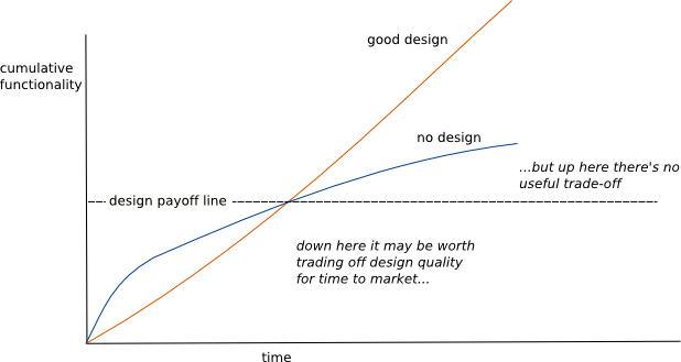
The remarkable thing about this graph is that it is based on no data as Martin Fowler candidly admits in his blog post and presentations (see for example the third mini-talk, about 45:00, in Software Development in the 21st Century by Martin Fowler). Yes, that is right: no data. 🙂 It is a hypothesis, a conjecture, but one held by Martin Fowler and strongly, even fanatically held by many software engineers and other technical professionals.

It is hard to define the terms in the design stamina hypothesis. In particular, what is “good design?” This often refers to a beautiful, modular system of software that is allegedly “scalable and maintainable”. Also the modules are allegedly reusable. I have certainly had the experience of trying to work with modular software that was neither scalable nor maintainable nor reusable and yet seemed to follow the common tenets of “good design.”

The hypothesis also sets up a straw man. True “no design” is actually pretty rare in professional software development. Rather the real debates are between “good design” (my design) and “less good design” (your design, also known as !@#$%). Or between “more time spent on design” (product ship date is one year away) and “less time spent on design” (product ship date is two weeks away).

Actual Data

Martin Fowler begs off on producing actual data to back up his pseudo-graph. In highly technical, highly mathematical areas of software development, it is often possible to define objective performance metrics that correspond closely to the business value of the products or services.

In speech recognition a good objective performance metric is the word recognition accuracy of the speech recognition engine; a speech recognition engine that recognizes ninety-five percent of spoken words is better than one that recognizes ninety percent.

In video compression, one of the key objective performance metrics is the compression ratio which is simply the size of the video before it is compressed divided by the size of the video after it is compressed. This translates directly into lower storage costs, more channels of video for a cable system or YouTube, and so on. It is not hard to relate it directly to the dollar business value that financial analysts (bean-counters) care about.

Here is a graph of the compression ratio, the performance, of the best video compression technologies in the world versus time:

Actual Data

Video compression improved very little between 1995 and 2003. This was actually a period of wide-open competition in video codecs (codec stands for encoder/decoder or compressor/decompressor) because Microsoft, despite its reputation, provided an open architecture through Video for Windows and MCI (Media Control Interface) that enabled third party developers to rapidly integrate any video or audio compression algorithm into the then universal Windows operating system. In fact, hundreds of video codecs proliferated during this period. But the bit rate for minimum usable video remained stuck at about 1 Megabit per second.

Suddenly, video compression leaped forward during 2003, in just a matter of months. The new advances were quickly copied by many video codecs. The bit rate for minimum usable video dropped from one megabit per second to around 275 kilobits per second — lower for some “talking heads” video that is easier to compress.

This dramatic technical advance remains largely unnoticed by the general public! It in fact enabled YouTube, Skype, and the proliferation of video on the Internet since 2003.

Then, the compression ratio went flat again. In fact, there was negligible progress until 2008. The early “high performance” video codecs such as H.264/AVC (Advanced Video Coding) had some problems properly reproducing skin tone, which is noticeable since people generally look at faces. In my graph, I use a different color from 2008 onwards to show the improvement in skin tone and perceived quality although the compression ratio did not change significantly.

What does this tell us about the design stamina hypothesis? Were the video codecs the product of “no design” from 1995 (actually earlier) to 2003? Did they suddenly switch over to “good software design” for a few brief months in 2003? Then the crazed cowboy coders took over again in 2004, inflicting “no design” until a brief shining moment in 2008 when the agile software designers took over again before being ousted in a violent coup by the cowboy coders?

Clearly, the actual performance curves bear little resemblance to the beautiful “good design” and “no design” curves in the design stamina hypothesis pseudo-graph. In fact, they resemble the famous “technology S-curve” postulated by students of the history of technology, invention and discovery.

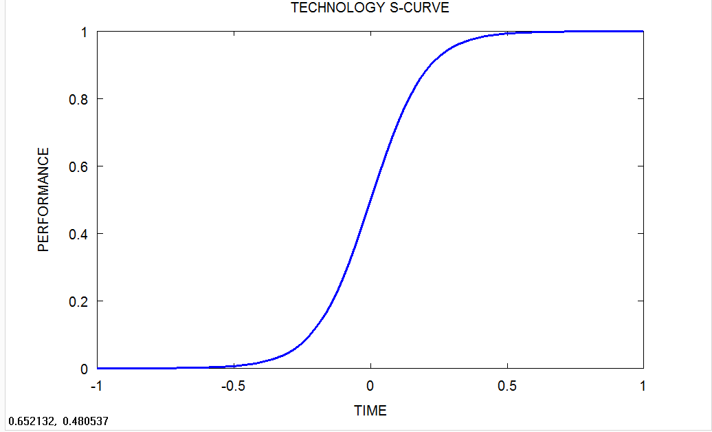
Technology S Curve

The basic idea behind the Technology S Curve is that technologies tend to go through a period of slow development during their early stages, a period of rapid development when the new technology gets past the proof of concept stage, and then slow down and often plateau when technical limits, often from fundamental physics or mathematics are encountered.

In aviation, propeller planes eventually topped out in speed. Jets were needed to go faster, break the sound barrier. Chemical rockets are faster but top out at several miles per second due to the constraints of the rocket equation and known materials. In principal, nuclear rockets could go faster. Fusion propulsion even faster. Antimatter rockets might be able to reach near the speed of light and travel to the nearest stars.

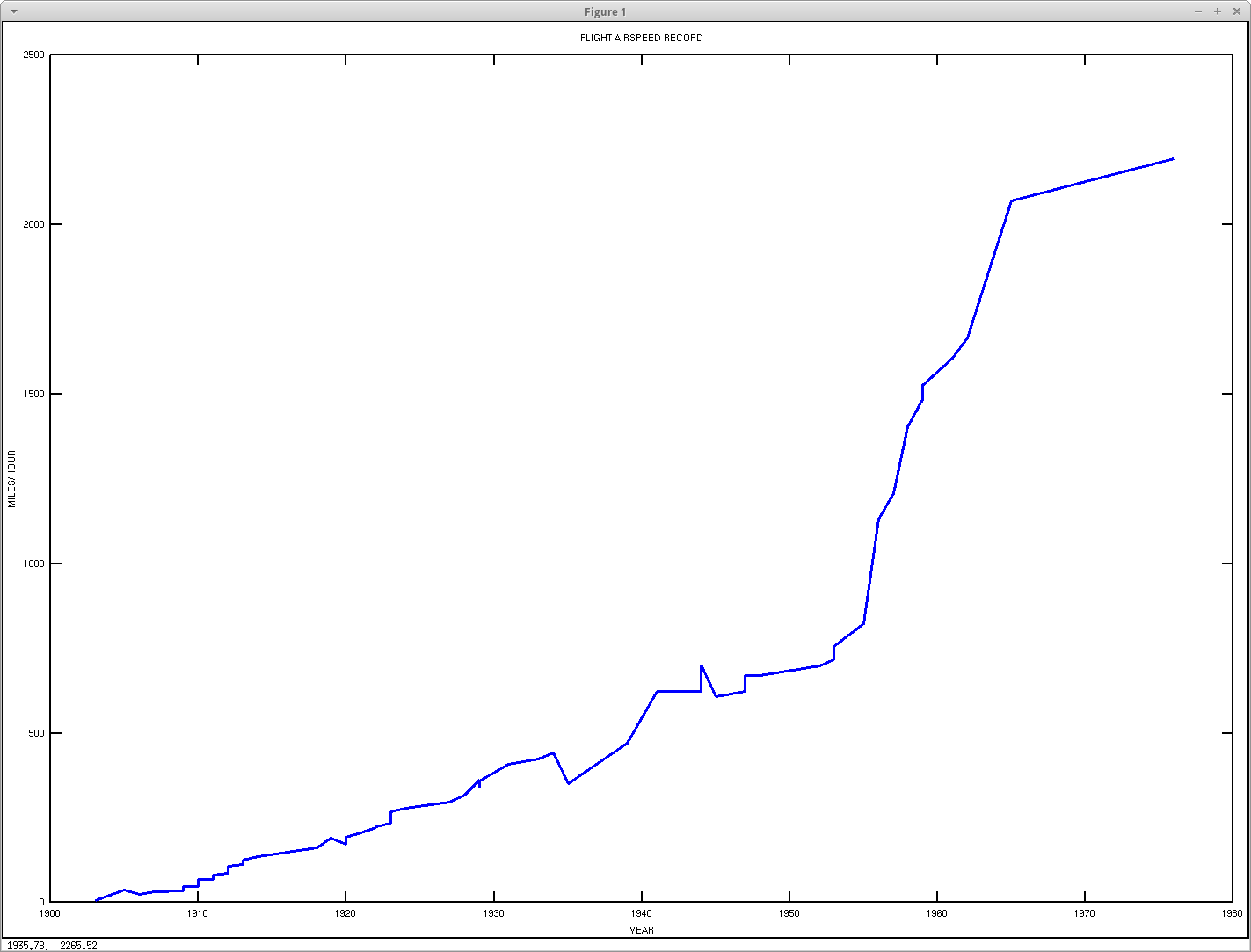
Flight Airspeed Record Data (Source: Wikipedia)

NOTE: Above graph added to post on July 18, 2014 — after first publication. The data is the flight airspeed record data from Wikipedia (accessed on July 18, 2014). See the appendix for the GNU Octave Code and cleaned data from the Wikipedia page used to generate the graph. The sharp climb in the 1950’s is due to the introduction of jet engines. Note also that the top speed of propeller planes is roughly linear with year — not an idealized S-curve. The final top speed record is for the SR-71 Blackbird spy plane — still officially the top record speed for a jet aircraft.

Each technology plateaus at some point and something new, sometimes a new component, sometimes a radical new architecture is needed. This gives rise to the technology S curve in many cases — not in all.

Heavily mathematical algorithms and software, like video compression, often seem to behave like this. Progress occurs in fits and starts, periods of no progress and sudden jumps, occasional periods of steady incremental progress. It often does not resemble the curves in the design stamina hypothesis pseudo-graph.

Leprechauns in the Measurement Free Zone

Software engineering and software design is a remarkably evidence-free field. One researcher has described it as “The Measurement Free Zone.” This is all the more remarkable given the high intelligence and technical backgrounds of the software design theorists and practitioners.

A few years ago Agile software development enthusiast Laurent Bossavit wrote an online book The Leprechauns of Software Engineering: How folklore turns into fact and what to do about it detailing his research into the basis for a number of common, heavily cited beliefs in software engineering, beliefs which he had held. He has also written an article on his experience for Model View Culture web site: The Making of Myths. The beliefs often turn out to be based on very limited evidence, open to alternative interpretation, or even pseudo-graphs like Fowler’s Design Stamina Hypothesis that illustrate not data but simply a personal belief, perhaps based on some undocumented personal experience.

Undocumented personal experience is also known as “anecdotal evidence” and anathema, with some justification, in the mainstream scientific and professional engineering literature. I don’t entirely agree with this mainstream taboo, but one should certainly be cautious with “anecdotal evidence.”

When I investigated the epidemic of autism in the United States (see The Mathematics of Autism), I found many accounts by parents of autism or at least behavioral problems diagnosed as autism occurring in conjunction with vaccinations. These are often very specific. My kid received the MMR (Measles-Mumps-Rubella) vaccine at about 18 months, had a reaction to the vaccine, and then stopped speaking and began to exhibit odd behavior leading to a diagnosis of autism. These are direct, specific personal experience and many parents are quite certain that the vaccines somehow caused the autism.

The “you read Andrew Wakefield’s articles and are just imagining it after the fact” explanations by the CDC and medical-scientific establishment, adamantly and financially committed to vaccines, aren’t particularly convincing or credible. But is it true? Do vaccines cause autism or is there some other explanation for these experiences?

In the technology S-curve, if you happen to be involved in a project during the middle rapid-progress period, it will look exactly like Martin Fowler’s “good design” curve. On the other hand, if you are involved later in the project, starting near or after the end of the rapid progress period, it will look exactly like the “no design” curve.

Often as technologies reach the plateau, they become very complicated. This complexity however buys very small or no improvements in performance. The technology is simply reaching its limits and it takes an awful lot to squeeze a little more out of it. At this point, a technology that is becoming complicated in this way may genuinely resembles “no design,” spaghetti code, inexplicably complicated to a newcomer.

In fact, a high performance video codec like the free open-source x264 is extremely complex.

Joel Spolsky wrote a widely-read, widely ignored blog post Things You Should Never Do about the bizarre and often disastrous tendency of software engineers to try to rewrite shipping, successful software — from scratch in many cases. Software marketing expert Merrill R. (Rick) Chapman describes several cases of this at companies he worked for in the 1980’s in his book In Search of Stupidity: Over Twenty Years of High Tech Marketing Disasters. Not infrequently the attempt to rewrite the “bad code” takes an extremely long time or fails outright, by which time a competitor has overtaken the company with new features in a competing product that was not rewritten or refactored in modern parlance.

In most of these cases, the rewriters or refactorers encounter an extremely complex confusing code base presumably written by highly paid professional software developers who have either cashed in their stock options and are now playing golf in Maui or have been downsized without reward by their heartless employer in favor of younger, presumably smarter developers trained in the latest software design methodology. 🙂 The obvious conclusion is that the working software was built with “no design.” Could Martin Fowler and the Design Stamina Hypothesis be wrong?

A Call for Data

The Design Stamina Hypothesis is admittedly not based on data. It is a hypothesis, a conjecture. Martin Fowler clearly admits this — to his credit. Martin Fowler didn’t really invent this concept. I have heard some variant of it for over twenty years (the blog post is dated 2007) especially from advocates of various software design methodologies (structured design in the 1980’s, object-oriented design in the 1990’s, Agile and Lean and XP and so on in the 00’s).

Where is the data?

It is possible to construct objective performance metrics like the compression ratio that correspond closely to business value, certainly in highly technical, mathematical software like video compression or speech recognition.

There are probably similar objective performance metrics in business software. For example, the number of transactions per second that a business software system — payroll, order entry, etc. — can process. These can be plotted against time and effort. One can certainly measure roughly the amount of time spent on design versus coding, testing, or other activities. Does the data actually show the curves in the Design Stamina Hypothesis, technology S-curves, something else, or a lot of confusion?

The benefits of such evidence-based decision making may well include avoiding making the expensive and often fatal mistake of attempting to rewrite or refactor an extremely complex product or system that is extremely complex for good reasons such as the plateau at the end of the technology S-curve.

© 2014 John F. McGowan

About the Author

John F. McGowan, Ph.D. solves problems using mathematics and mathematical software, including developing video compression and speech recognition technologies. He has extensive experience developing software in C, C++, Visual Basic, Mathematica, MATLAB, and many other programming languages. He is probably best known for his AVI Overview, an Internet FAQ (Frequently Asked Questions) on the Microsoft AVI (Audio Video Interleave) file format. He has worked as a contractor at NASA Ames Research Center involved in the research and development of image and video processing algorithms and technology. He has published articles on the origin and evolution of life, the exploration of Mars (anticipating the discovery of methane on Mars), and cheap access to space. He has a Ph.D. in physics from the University of Illinois at Urbana-Champaign and a B.S. in physics from the California Institute of Technology (Caltech). He can be reached at [email protected].

Appendix: Octave Code for Figures

%
% (C) 2014 by John F. McGowan, Ph.D.
%
% rough plot of improvements in video compression performance over time
%
% compare to: https://martinfowler.com/bliki/DesignStaminaHypothesis.html
%
%  --  https://martinfowler.com/bliki/images/designStaminaGraph.gif

% plateau's or near plateaus in video compression performance
%
period1 = 1995:2002;  % THE MPEG ERA
period2 = 2003:2007;  % THE BREAKTHROUGH IN 2003  (H.264 etc.)
period3 = 2008:2014;  % ADVANCES IN REPRODUCING SKIN TONES 2008/2009

frame_rate = 30;  % frames per second (NTSC is technically 29.97 frames/second)
bits_per_byte = 8;
color_channels_per_pixel = 3;  % usually YCrCb (Y is black/white signal, Cr and Cb carry color)
width = 720;
height = 480;

uncompressed_rate = width*height*color_channels_per_pixel*bits_per_byte*frame_rate;
mpeg1_rate = 1000000;  % one megabit per second
h264_rate = 275000;    % 275 kilobits per second (also Ogg Theora, Windows Media, Silverlight)

% perceived quality is close to old analog NTSC television
% under excellent broadcast conditions (lower than DVD or BluRay playback)
% DVD is MPEG-2 with bit rate of 4-8 Megabits per second (same core technology as MPEG-1)
%

% compute compression ratio for periods
cr1 = (uncompressed_rate / mpeg1_rate)*ones(size(period1));
cr2 = (uncompressed_rate / h264_rate)*ones(size(period2));
cr3 = (uncompressed_rate / h264_rate)*ones(size(period3));

% plot compression ratio over time
%
figure(1);
plot(period1, cr1, "1", "linewidth", 3,
period2, cr2, "2", "linewidth", 3,
period3, cr3, "3", "linewidth", 3);

title('VIDEO COMPRESSION PERFORMANCE');
xlabel('YEAR');
ylabel('COMPRESSION RATIO');
legend('MPEG-1 ERA', 'H.264 ERA', 'BETTER SKIN TONE', 'location', 'southeast');

% make plot for technology S-CURVE
%
figure(2);
x = -1.0:0.02:1.0;
y = 1.0 ./ (1.0 + exp(-1.0*10.0*x));
plot(x,y, "linewidth", 3);
title('TECHNOLOGY S-CURVE');
xlabel('TIME');
ylabel('PERFORMANCE');


% THE END

airspeed_scurve.m

%
% make plot for maximum airspeed technology S-curve
%

% data from Wikipedia
% https://en.wikipedia.org/wiki/Flight_airspeed_record
%
% 

data = dlmread('airspeed_cleaned.txt', '\t');
year = data(3:end, 1);  % date/year
mph  = data(3:end, 3);  % miles per hour of record
kph  = data(3:end, 4);  % kilometers per hour of record

plot(year, mph);
xlabel('YEAR');
ylabel('MILES/HOUR');
title('FLIGHT AIRSPEED RECORD');

airspeed_cleaned.txt

Date 	Pilot 	Airspeed 	Aircraft 	Location 	Notes
mph 	km/h
1903 	Wilbur Wright 	6.82 	10.98 	Wright Flyer 	Kitty Hawk, North Carolina, USA 	
1905 	Wilbur Wright 	37.85 	60.23 	Wright Flyer III 		
1906 	Alberto Santos-Dumont 	25.65 	41.292 	Santos-Dumont 14-bis 	Bagatelle Castle, Paris, France 	First officially recognized airspeed record. [2] [3]
1907 	Henry Farman 	32.73 	52.700 	Voisin-Farman I 	Issy-les-Moulineaux, France 	[2] [4]
1909 	Paul Tissandier 	34.04 	54.810 	Wright Model A 	Pau, France 	[2] [5]
1909 	Glenn Curtiss 	43.367 	69.821 	Curtiss No. 2 	Reims, France 	1909 Gordon Bennett Cup. [2] [6]
1909 	Louis Blériot 	46.160 	74.318 	Blériot XI 	Reims, France 	[2] [7]
1909 	Louis Blériot 	47.823 	76.995 	Blériot XI 	Reims, France 	[2] [7]
1910 	Hubert Latham 	48.186 	77.579 	Antoinette VII 	Nice, France 	[2] [8]
1910 	Léon Morane 	66.154 	106.508 	Blériot 	Reims, France 	[2] [7]
1910 	Alfred Leblanc 	68.171 	109.756 	Blériot XI 	New York, New York, USA 	[2] [7]
1911 	Alfred Leblanc 	69.442 	111.801 	Blériot Blériot 	Pau, France 	[2] [9]
1911 	Édouard Nieuport 	73.385 	119.760 	Nieuport IIN 	Châlons, France 	[2] [10]
1911 	Alfred Leblanc 	77.640 	125.000 	Blériot 		[2]
1911 	Édouard Nieuport 	80.781 	130.057 	Nieuport IIN 	Châlons, France 	[2] [10]
1911 	Édouard Nieuport 	82.693 	133.136 	Nieuport IIN 	Châlons, France 	[2] [10]
1912 	Jules Védrines 	87.68 	145.161 	Deperdussin Monocoque (1912) 	Pau, France 	[2] [11]
1912 	Jules Védrines 	100.18 	161.290 	Deperdussin monoplane 	Pau, France 	[2] [11]
1912 	Jules Védrines 	100.90 	162.454 	Deperdussin Monocoque 	Pau, France 	[2] [11]
1912 	Jules Védrines 	103.62 	166.821 	Deperdussin Monocoque 	Pau, France 	[2] [11]
1912 	Jules Védrines 	104.29 	167.910 	Deperdussin Monocoque 	Pau, France 	[2] [11]
1912 	Jules Védrines 	106.07 	170.777 	Deperdussin Monocoque 	Reims, France 	[2] [11]
1912 	Jules Védrines 	108.14 	174.100 	Deperdussin Monocoque (1912) 	Chicago, Illinois, USA 	[2] [11]
1913 	Maurice Prévost 	111.69 	179.820 	Deperdussin Monocoque (1913) 	Reims, France 	[2] [12]
1913 	Maurice Prévost 	119.19 	191.897 	Deperdussin Monocoque (1913) 	Reims, France 	[2] [12]
1913 	Maurice Prévost 	126.61 	203.850 	Deperdussin Monocoque (1913) 	Reims, France 	[2] [12]
1914 	Norman Spratt 	134.5 	216.5 	Royal Aircraft Factory S.E.4 		Unofficial
1918 	Roland Rohlfs 	163 	262.3 	Curtiss Wasp 		Not officially recognised.[13]
1919 	Joseph Sadi-Lecointe 	191.1 	307.5 	Nieuport-Delage NiD 29V 		Not officially recognised.
1920 	Joseph Sadi-Lecointe 	171.0 	275.264 	Nieuport-Delage NiD 29V 	Villacoublay, France. 	[14] First official record post World War 1. [2] [15]
1920 	Jean Casale 	176.1 	283.464 	Spad-Herbemont 20 bis 	Villacoublay, France 	[2] [16] [17]
1920 	Bernard de Romanet 	181.8 	292.682 	Spad-Herbemont 20 bis 	Buc, France 	[2] [18] [17]
1920 	Joseph Sadi-Lecointe 	184.3 	296.694 	Nieuport-Delage NiD 29V 	Buc, France 	[2] [15]
1920 	Joseph Sadi-Lecointe 	187.9 	302.529 	Nieuport-Delage NiD 29V 	Villacoublay, France 	[2] [15]
1920 	Bernard de Romanet 	191.9 	309.012 	SPAD S.XX 	Buc, France 	[2][19]
1920 	Joseph Sadi-Lecointe 	194.4 	313.043 	Nieuport-Delage NiD 29V 	Villacoublay, France 	[2] [15]
1921 	Joseph Sadi-Lecointe 	205.2 	330.275 	Nieuport-Delage Sesquiplane 	Ville Sauvage, France 	[20] [21]
1922 	Billy Mitchell 	222.88 	358.836 	Curtiss R 	Detroit, Michigan, USA 	[2] [22]
1922 	Billy Mitchell 	224.28 	360.93 	Curtiss R-6 	Selfridge Field, Detroit, Michigan, USA 	[23] [24] [25]
1923 	Joseph Sadi-Lecointe 	232.91 	375.00 	Nieuport-Delage 	Istres 	[22]
1923 	1st Lt. Russell L. Maughan 	236.587 	380.74 	Curtiss R-6 	Wright Field, Dayton, Ohio, USA 	[26] [27] [25]
1923 	Lt. Harold J. Brow 	259.16 	417.07 	Curtiss R2C-1 	Mineola, New York, USA 	[28] [29]
1923 	Lt. Alford J. Williams 	266.59 	429.02 	Curtiss R2C-1 	Mineola, New York, USA 	[28][30] [29]
1924 	Florentin Bonnet 	278.37 	448.171 	Bernard-Ferbois V.2 		[2]
1927 	Mario de Bernardi 	297.70 	479.290 	Macchi M.52 seaplane 	Venice 	Database ID 11828 [1][2]
1928 	Mario de Bernardi 	318.620 	512.776 	Macchi M.52bis seaplane 	Venice 	Database ID 11827 [1][31]
1929 	Giuseppe Motta 	362.0 	582.6 	Macchi M.67 seaplane 		Unofficial
1929 	George H. Stainforth 	336.3 	541.4 	Gloster VI seaplane 	Calshot 	Database ID 11829[1][32]
1929 	Augustus Orlebar 	357.7 	575.5 	Supermarine S.6 seaplane 	Calshot 	Database ID 11830 [1][33]
1931 	George H. Stainforth 	407.5 	655.8 	Supermarine S.6B seaplane 	Lee-on-the-Solent 	Database ID 11831 [1][34]
1933 	Francesco Agello 	423.6 	682.078 	Macchi M.C.72 seaplane 	Desenzano del Garda 	Database ID 11836 [1][2]
1934 	Francesco Agello 	440.5 	709.209 	Macchi M.C.72 seaplane 	Desenzano del Garda 	Database ID 4497 [1][2]
1935 	Howard Hughes 	352 	566 	Hughes H-1 Racer landplane 		Not an Official FAI record
1939 	Fritz Wendel 	469.220 	755.138 	Me 209 V1 	Augsburg 	Piston-engined record until 1969[35]
1941 	Heini Dittmar 	623.65 	1003.67 	Messerschmitt Me 163A V4 	Peenemünde 	Rocket powered – Not an Official FAI record but over the 3 km FAI distance[36] [37][38]
1944 	Heinz Herlitzius 	624 	1004 	Messerschmitt Me 262 S2 	Leipheim 	Not an Official FAI record [39]
1944 	Heini Dittmar 	702 	1130 	Messerschmitt Me 163B V18 	Lagerlechfeld 	Rocket powered – Not an Official FAI record [39]
1945 	H. J. Wilson 	606.4 	975.9 	Gloster Meteor F Mk 4 	Herne Bay, UK 	EE455 Britannia, a Mk 3 converted on production line to a long-span Mk 4.[41]
1946 	Edward Mortlock Donaldson 	615.78 	990.79 	Gloster Meteor F Mk 4 	Littlehampton, UK 	EE530, a long-span Mk 4.[41]
1947 	Col. Albert Boyd 	623.74 	1003.60 	Lockheed P-80R Shooting Star 	Muroc, California, US 	[42]
1947 	Cmdr. Turner Caldwell 	640.663 	1031.049 	Douglas Skystreak 	Muroc, California, US 	[43]
1947 	Major Marion Eugene Carl USMC 	650.796 	1047.356 	Douglas Skystreak 	Muroc, California, US 	[43]
1947 	Chuck Yeager 	670.0 	1078 	Bell X-1 	Muroc, California, US 	Rocket powered – Not an official FAI C-1 record
1948 	Maj. Richard L. Johnson, USAF 	670.84 	1079.6 	North American F-86A-3 Sabre 	Cleveland, US 	[2] [44]
1952 	J. Slade Nash 	698.505 	1124.13 	North American F-86D Sabre 	Salton Sea, US 	[45]
1953 	William Barnes 	715.745 	1151.88 	North American F-86D Sabre 	Salton Sea, US 	[46]
1953 	Neville Duke 	727.6 	1171 	Hawker Hunter Mk.3 	Littlehampton, UK 	[47]
1953 	Mike Lithgow 	735.7 	1184 	Supermarine Swift F4 	Castel Idris, Tripoli, Libya 	[48]
1953 	James B. Verdin, US Navy 	752.9 	1211.5 	Douglas F4D Skyray 	Salton Sea, US 	[49]
1953 	Frank K. Everest USAF 	755.1 	1215.3 	North American F-100 Super Sabre 	Salton Sea, US 	
1955 	Horace A. Hanes 	822.1 	1323 	North American F-100C Super Sabre 	Palmdale, US 	
1956 	Peter Twiss 	1132 	1822 	Fairey Delta 2 	Chichester, UK 	[50]
1957 	USAF 	1207.6 	1943.5 	McDonnell F-101A Voodoo 	Edwards Air Force Base, US 	[51]
1958 	Cap. WW Irwin, USAF 	1404 	2259.5 	Lockheed YF-104A Starfighter 	Edwards Air Force Base, US 	[52]
1959 	Col. Georgii Mosolov 	1484 	2388 	Ye-66 (Mikoyan-Gurevich MiG-21) 	USSR 	[53]
1959 	Maj. Joseph Rogers, USAF 	1525.9 	2455.7 	Convair F-106 Delta Dart 	Edwards Air Force Base, US 	
1961 	Robert G. Robinson, US Navy 	1606.3 	2585.1 	McDonnell-Douglas F4H-1F Phantom II 	Edwards Air Force Base, US 	[54] [55]
1962 	Lt. Col. Georgii Mosolov 	1665.9 	2681 	Mikoyan Gurevich Ye-166 – name adopted for the record attempt, originally a version of a Ye-152 	USSR 	[35] [56] a.k.a. E-166.[57]
1965 	Robert L. Stephens and Daniel Andre 	2070.1 	3331.5 	Lockheed YF-12A 	Edwards AFB, US 	[58]
1976 	Capt. Eldon W. Joersz and Maj. George T. Morgan 	2193.2 	3529.6 	Lockheed SR-71 Blackbird #61-7958 	Beale AFB, US 	[59]