Prediction is very difficult, especially about the future.
Common quotation, variously attributed to Yogi Berra, Niels Bohr, Mark Twain and others.
Introduction
In Isaac Asimov’s famous science fiction novel Foundation, a group of scientists in the distant future led by Hari Seldon discover a mathematical method to predict the course of future events, anticipating the collapse of the reigning Galactic Empire into a new Dark Age. Armed with the mathematical methods of Hari Seldon’s “psychohistory,” the scientists create a Foundation on the edge of the Galaxy that saves civilization from the prophesied Dark Age. The notion that mathematics can be used to predict human behavior in economics, finance, politics, and many other fields and activities has great appeal. With the spread of increasingly powerful computers, complex mathematical models of economics, finance, and other human activities have become more and more common. Often, the motives are much less admirable than the selfless super scientists of Asimov’s tale. Often, too, the accuracy and performance of the mathematical models has been much less impressive than Asimov’s fictional new science of psychohistory.
In the last few years, complex models of the value of mortgage backed securities have proven disastrously incorrect, a major contributing factor to the Great Recession, the present financial crisis. This is only the latest in a succession of such failures in quantitative finance. Similarly, many sophisticated econometric models of the economy have proven unreliable. To the extent that these models are shaping public policy, personal and corporate investment decisions, and so forth, the pitfalls of mathematical modeling and seemingly abstruse issues in the philosophy of science such as Karl Popper‘s doctrine of falsifiability are having a substantial impact on people and society.
In fact, applying mathematical models to economics, finance, and other human activities is especially treacherous. All mathematical modeling suffers from the deep problem that one can construct an infinite range of functions that approximate current observations and data arbitrarily well and yet make any and all possible predictions about possible new observations. In practice, human beings use various criterion to select mathematical models that are likely to be true, many of which criterion cannot be justified in any rigorous or rational way and some of which criterion are difficult to identify (intuition, “that just doesn’t feel right”, “God doesn’t play dice with the universe.”). Nonetheless, human judgment has a high error rate, though surely much more accurate than a blind guess.
In addition to this pervasive problem, many of the assumptions used in applying mathematical models to physical processes such as the motion of the planets or radioactive decay surely do not apply to economics, finance, or other forms of human behavior. Our expectation is that the motion of the planets is governed by the same “laws” today as last year or last decade or in 1605 when Johannes Kepler first recognized the elliptical orbits of the planets. Indeed, this regularity of many natural phenomenon is strongly born out by experience. On the other hand, the economy or financial markets or other human activities change and evolve. However imperfectly, human beings learn from mistakes, develop new technologies and processes. Human beings are herd animals and prone to fads and fashions that have no parallel in physical phenomena. One would not expect the market for gold to be the same today as in 1960 and it was not. The price of gold was fixed by the US federal government in 1960 and today it is not.
This article takes a look at the price of gold since 1970 when the United States ended the gold standard. Gold is currently rising sharply in price as it did in the late 1970’s and early 1980’s. This article will show how it is possible to construct many different purely symbolic mathematical models of the price of gold that make different predictions. Indeed, one can cook up whatever prediction one would like. The article will also discuss the serious problems with applying the mathematical methods of physics and other “hard” sciences to the price of gold as a specific example of a general problem.
Mathematics for Goldfinger
With the collapse of the Bretton-Woods foreign exchange system (1968-1971), the price of gold, previously fixed to the US dollar, was allowed to float free. Since 1970 the price of an ounce of gold in US dollars has risen substantially.
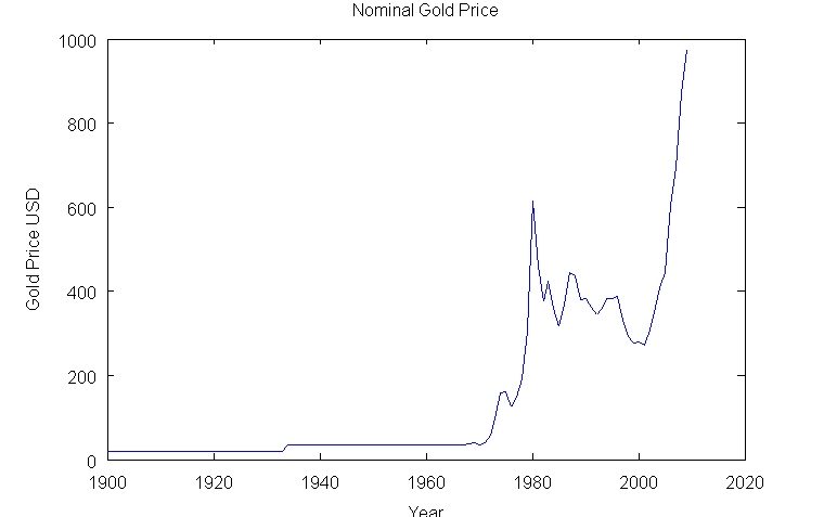
Nominal Gold Price
The United States government reports a consumer price index (CPI) that is purported to reflect the cost of living in US dollars for a typical US citizen. Although there are some reasons to be skeptical about the accuracy of the CPI in recent years, this article will use the CPI as a proxy for the overall price level in the United States.
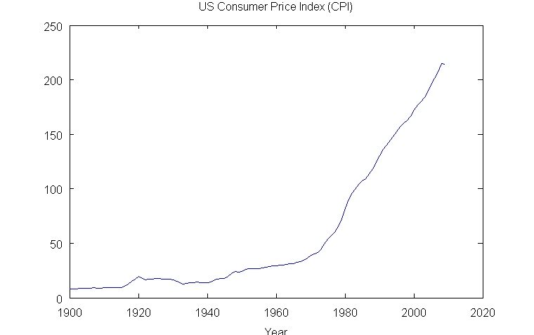
United States Consumer Price Index
One can see that the CPI has generally risen at a higher rate since the United States ended the gold standard in 1970. This also corresponds to a period of overall rising energy prices and very limited progress in power and propulsion technologies. Many other areas have seen relatively limited scientific and technological progress during this period. Computers and electronics have, of course, continued their historical trend of rapid progress to the present.
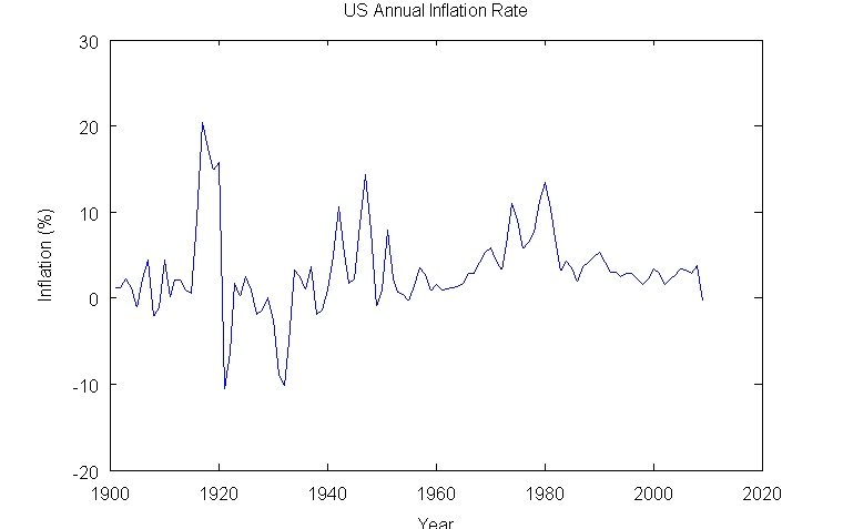
Historically, the US inflation rate was high during the periods of World War I and World War II, but otherwise generally lower than the present period, since 1970. The official inflation rate, the rate of increase of the CPI, was especially high during the 1970s, a period of sharp increases in nominal and real energy prices. The inflation rate derived from the CPI in recent years does not seem to reflect the common experience of rising energy prices since the late 1990s. Nor does it show any evidence of the sharp rise in housing prices in the US from 2002 to 2005; by many estimates, housing prices in urban areas remain high compared to the historical trend.

Inflation Adjusted Gold Price
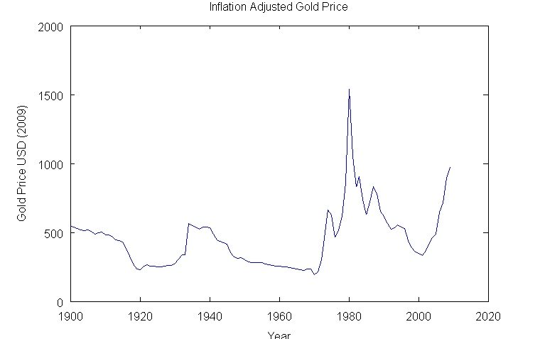
Investors are generally interested in the real inflation-adjusted value of an investment. The value of gold in real terms fluctuated somewhat during the period of the gold standard but has fluctuated much more since 1970. Particularly notable is the large spike in the real and nominal price of gold in the early 1980’s. In real terms, the current rise in gold price has not reached the level of the spike in the early 1980’s. If inflation has been higher than the official CPI, the current real price of gold would be even lower than the spike in the early 1980s.
One can construct a simple symbolic mathematical model of the real price of gold since 1970 (the gold standard disintegrated between 1968 and August 1971 when the US government ended any attempt to tie the dollar to gold) by using a polynomial with several terms:
[tex] \[\mathrm{p}\left( t\right) =c\,{t}^{2}+b\,t+a\] [/tex]
Where [tex]\mathrm{p}\left( t\right)[/tex] is the gold price as a function of the time [tex]t[/tex]. This is a simple mathematical model with little real-world justification. It will, in fact, make grossly unrealistic predictions that should call it into question. A polynomial model of the time series of real gold prices is:
[tex] \[\mathrm{p}\left( t\right) =l\,{t}^{11}+k\,{t}^{10}+j\,{t}^{9}+i\,{t}^{8}+h\,{t}^{7}\][/tex]
[tex]\[ + g\,{t}^{6}+f\,{t}^{5}+e\,{t}^{4}+d\,{t}^{3}+c\,{t}^{2}+b\,t+a\][/tex]
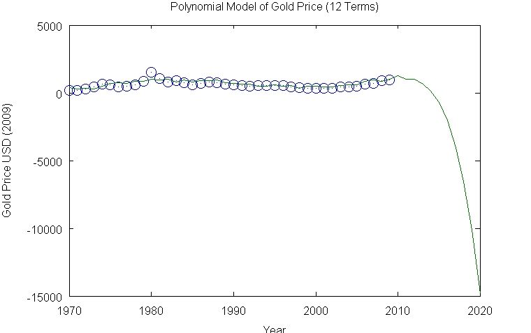
Polynomial Model of Gold Price (12 Terms)
One can approximate any continuous function as accurately as one would like with a sum of a series of powers. The problem is that a power such as [tex] t^{12} [/tex] will grow without bound as the independent variable [tex] t [/tex] grows. This is usually quite unrealistic. This is a simple illustration of the difference between a symbolic mathematical model of reality and our common sense every day sense of reality.
Apocalypse or Gold Bubble?
Many other mathematical models are possible. In fact, there are an infinite number of functions or curves that agree with the data during the period from 1970 to 2009. In this way, one can predict anything. In mathematical models of physical phenomenon, it is common to try to construct the model from a set of building block functions, or more generally terms such as terms in a differential equation. This may be arbitrary or justified by arguing that the building blocks represent fundamental building blocks of the physical process in some way. In practice, one is trying to capture regularities in the data that may recur in new data. For example, the position of a pendulum is periodic; it repeats over and over again. Simple harmonic motion of this type was one of the first kinds of behavior understood mathematically by the ancients. One can construct models of the gold price data that agree with the data quite well by eye using a collection of peaks rather than periodic functions. One might, for example, represent the seeming peaks in the gold price data as the Gaussian or Normal function, commonly referred to as the “Bell Curve,”
[tex]\[ N(t, \mu, \sigma) = \frac{1.0}{\sqrt{2\pi}\,\sigma} {{e}^{-\frac{1.0\,{\left( t-\mu\right) }^{2}}{{\sigma}^{2}}} }\][/tex]
A very simple model is the sum of two Gaussians:
[tex] \[\mathrm{p}\left( t\right) = A_1N(t,\mu_1,\sigma_1) + A_2 N(t, \mu_2, \sigma_2) \] [/tex]

Gold 2 Gaussian Model
This simple model with two Gaussians does not agree very well with the data. It predicts the following future performance:
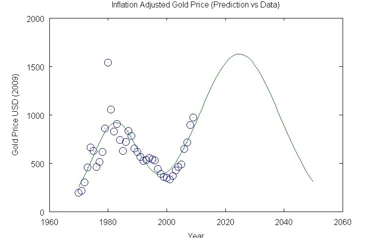
Gold 2 Gaussian Prediction
It predicts that the real price of gold will peak in about 2025 and then drop. One can get much better agreement between the model and the gold price data by adding more Gaussians, loosely corresponding to the apparent gold peaks in about 1974, 1982, 1987, 1993, and today. The spike in 1982 is especially sharp and can better be approximated by combining two Gaussians.
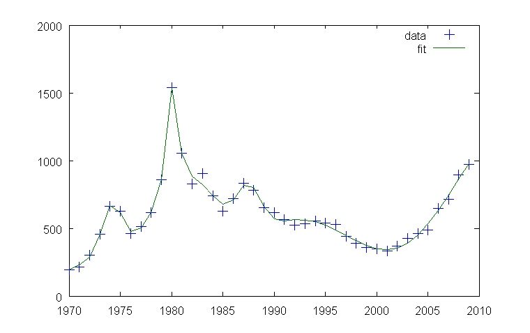
Gold 7 Gaussian Model
Now the agreement by eye is much better. The curves appear essentially the same. This model makes a different prediction.
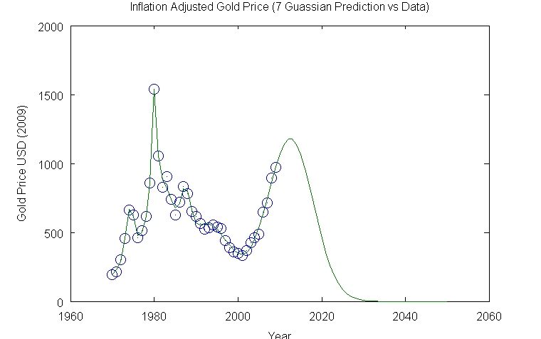
Gold 7 Gaussian Prediction
This model predicts a peak in real gold prices in just a few years, about 2012, followed by a decline to essentially zero. One can get significantly different predictions simply by using a different function to model the peaks in the gold price. For example, one can use the Cauchy-Lorentz distribution as a model for the peaks:
[tex]\[\mathrm{C}\left( t,\mu,\sigma\right) =\frac{1}{\frac{{\left( x-\mu\right) }^{2}}{{\sigma}^{2}}+1}\][/tex]
where [tex]t[/tex] is the time (year in this case), [tex] \mu [/tex] is the location of the peak, and [tex] \sigma [/tex] is a measure of the width or dispersion of the peak. Initially, one can try a model with two peaks:
[tex] \[\mathrm{p}\left( t\right) = A_1C(t,\mu_1,\sigma_1) + A_2 C(t, \mu_2, \sigma_2) \] [/tex]
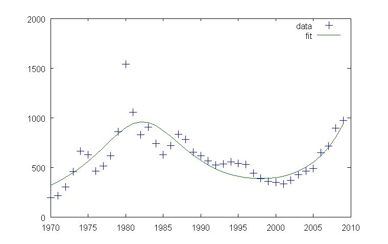
Gold 2 Cauchy Model
This model looks very similar to the two Gaussian model. It predicts something different however.
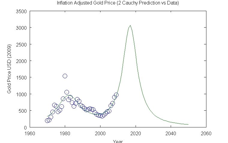
Gold 2 Cauchy Prediction
In this case, the price of gold trails off slowly instead of dropping to essentially zero in about a decade. This is a difference between the Gaussian and the Cauchy-Lorentz functions. Of course, the agreement between the model and data is not very good. One probably would not and should not trust it. One can achieve better agreement with more peaks, just as in the Gaussian models.
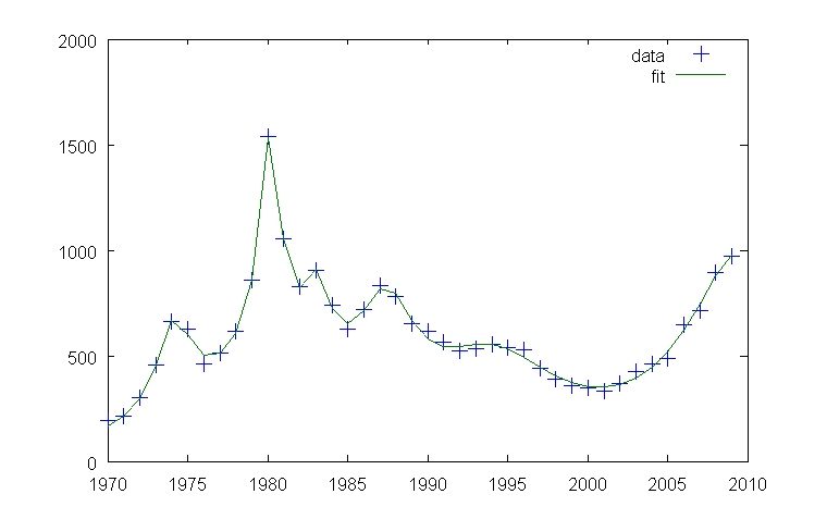
Gold 7 Cauchy Model
Now the agreement is almost exact by eye. The prediction however differs from the seven Gaussian model.
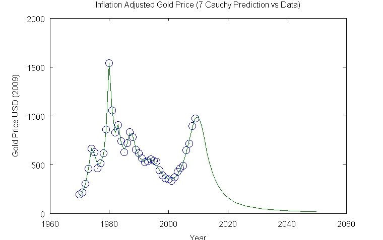
Gold 7 Cauchy Prediction
Again, the price of gold trails off slowly over a period of decades due to the difference between the Gaussian and Cauchy-Lorentz peak models. In fact, one can get essentially any prediction by choosing the appropriate mathematical model. How reasonable are these predictions? There are several theories about the present rise in gold prices. One clear contender is that the gold price rise in the last decade is yet another speculative financial bubble. In this scenario, one would expect the price of gold to drop substantially within a decade. One might also argue that the sharp run-up in gold prices will encourage overproduction of gold and the development of better gold refining, recycling technologies, alternatives to gold, and even perhaps the alchemist’s dream of converting base metals into gold (using nuclear reactors for example). At the other extreme, the rise in gold prices is tied to apocalyptic scenarios in which the US and other governments go bankrupt due to deficit spending and the dollar and other paper currencies becomes as valueless as the German mark during the infamous German hyperinflation. Thus, the real inflation-adjusted price of gold spikes as investors seek an inflation proof haven. Unfortunately, civilization collapses. Gold and other luxury items become valueless in the bitter Darwinian battle for survival in the post-apocalyptic world. The most valuable possessions are a gun, ammunition, and a large horde of dried food — all purchased from advertisers on Alex Jones web site. In either scenario, gold eventually tanks.
All kidding aside, it is usually possible to find technically sophisticated, plausible justifications for mathematical models. Usually does not mean always. The behavior of the polynomial models is grossly unrealistic. How likely is it that the price of gold would go negative, let alone extremely negative — meaning that people would be paying large sums of money to get rid of gold? The evidence that the Earth is nearly spherical with a diameter of about 8000 miles is very strong. Any argument that the Earth is really flat is extremely difficult to make in the present day. Most of us are pretty confident that the Sun will set today and rise again tomorrow and continue to do so for many, many years to come. There is some knowledge that is pretty certain. There are some mathematical models that have proven extremely accurate and reliable.
Nonetheless, it is usually possible to find plausible arguments for mathematical models and conceptual theories. One can usually explain away even grossly contradictory — “falsifying” in the language of Karl Popper — observations or experiments in a technically sophisticated, plausible way. This can create the illusion that a theory or mathematical model falls into the category of almost certain knowledge, our common sense notion of a fact. Once upon a time, many people believed that it was a fact that the Earth was flat. How could it possibly be a sphere? Political power, social status, and sizable funding tend to flow to those who claim certainty, to know hard facts rather than speculative theories. In common thinking, an expert is someone who says “I know the answer.” not someone who says “I don’t know.”
Scientists and science popularizers often seek to promote reigning scientific theories to the level of “almost certain” knowledge or “facts,” such as that the Earth is roughly spherical or the historical fact of the Holocaust. These latter two are the most common analogies cited in the popular science literature. Scientific theories are said to be supported by “overwhelming evidence.” There is a “consensus” that the theory is correct. The theory is no longer a theory, but a fact. In debates about evolution and creation, one encounters the curious claim that evolution is a falsifiable theory, that creationism or “intelligent design” is not falsifiable and thus not scientific, and that evolution is also a fact beyond any reasonable dispute or falsification. Increasingly, malcontents or die-hards who question the “consensus” are “deniers” or “denialists” in analogy to Holocaust deniers, an extremely emotional analogy indeed. There are now evolution deniers, AIDS deniers, global warming deniers, and a growing list of other deniers. Yet, certain knowledge is relatively rare especially in the frontiers of science.
In the case of gold, one can make a strong argument that the models above are unlikely to be correct. There is a certain fundamental demand for gold for industrial uses, in electronics for example. There is a long history of people buying gold for jewelry. The economic and political problems, the fears and the greed, that have historically driven the fluctuations in the price of gold are likely to continue through the 21st century. Thus, one should doubt models that show the real price of gold dropping to zero or nearly zero. Yet, both symbolic mathematics and verbal reasoning enable one to make a plausible argument that this will happen, supported by fancy symbolic mathematics and technical graphs.
A Deep Problem
It is always possible to perfectly match or fit any set of [tex]N[/tex] data points using a linear combination of at least [tex]N[/tex] linearly independent functions. Under many conditions, a function or composition of building block functions with [tex]N[/tex] adjustable parameters can also match or fit any set of [tex]N[/tex] data points. In addition, with creativity and trial and error, one can often construct mathematical models with less than [tex]N[/tex] parameters or building block functions that nonetheless do a good job of matching or fitting [tex]N[/tex] data points. These models may often fail to predict future data or data that lies outside of the region used to make the model or fit.
In general, a composition of a set of building block functions has a sort of plasticity, a certain ability to match any data to some degree. If there are [tex]N[/tex] building block functions or adjustable parameters and [tex]N[/tex] data points, this plasticity can be rigorously shown to be essentially infinite, that is the model can always match any set of [tex]N[/tex] data points. The philosopher of science Karl Popper called such models or theories unfalsifiable. They can never be proven wrong. They predict everything and therefore they also predict nothing. Unlike popular presentations of his doctrine of falsifiability, Popper recognized that falsifiability was often not a black and white distinction. There were degrees of falsifiability and he tried to define some logical and quantitative criterion for the degree of falsifiability. What this means is that a mathematical model or theory with [tex]M[/tex] adjustable parameters where [tex]M[/tex] is less than the number of data points [tex]N[/tex] may still match a broad class of possible observations or data. It can be falsified, perhaps, but only with great difficulty. There is, in the examples above, a lot of freedom to match many different sets of data with seven peaks in the model. The models have 21 adjustable parameters and there are 40 data points (40 years). Although the models cannot exactly match all sets of 40 data points, nonetheless they are likely to be good enough for most purposes. Remaining differences between the data and the models can easily be attributed to noise, measurement errors, or some similar excuse.
In physics, there are some examples of very large data sets that match very simple mathematical formulas. The motions of the planets in the Solar System conform to Kepler’s Laws and Newton’s theory of gravitation to a very high degree. This is not necessarily true for the motion of stars in the Milky Way galaxy, galaxies in galactic clusters and so forth. A deviation from Newtonian gravity is a possible explanation for the anomalies often cited as evidence for so-called “dark matter” or “dark energy.” So too, there is an enormous amount of quantitative data on the vibration of springs and strings, the motion of pendulums, simple radioactive decays, and various other physical phenomena that show precise matches to simple mathematical expressions such as Hooke’s Law for springs or exponential decay for radioactive decay. It is fair to say that the amount of data points is now in the millions or more and the models have only a few adjustable parameters such as the half-life of a radioactive isotope. Consequently, it is probably reasonable to have a high degree of confidence in these models. At the other extreme, it is clear that we should put no confidence in the predictive power of models with as many adjustable parameters or building block functions as the number of data points.
In many situations however including the frontiers of human knowledge and often areas like economics, the situation falls into a gray area. The theories, both symbolic mathematical models and conceptual models, may be complex, but not so complex as to be obviously “unfalsifiable.” The amount of data may be limited or of questionable quality, but still not obviously inadequate to draw conclusions. It is here that faulty human judgment is in practice applied, in part because human judgment, fallible though it undoubtedly is, is still the best option, more reliable than symbolic mathematics or computer programs in many cases. In constructing mathematical models in these cases, human judgment is often hidden in the definition of the symbols and the choice of building block functions or other mathematical components used in the model.
Economics, finance, politics and other human activities are especially treacherous areas for mathematical modeling. The mathematical and scientific methods used in physics and other “hard” sciences were developed to study highly repeatable phenomena that do not appear to change appreciably over time. For example, a “fair” coin will come up heads when flipped on average half the time, tails half the time. This was true in the early days of probability and statistics during the Renaissance. It is true today. Fair games of chance work the same way today as yesterday, last year, last century, and presumably thousands of years ago or in the future. One can collect vast amounts of data on these games. Similarly, physical phenomena such as the motion of the planets, radioactive decay, and so forth appear to behave the same way time after time. They do not evolve, learn from mistakes, forget lessons learned, or suddenly change for difficult to understand reasons. None of this is true of much economic or financial data.
In the example of gold, the behavior of gold changed radically from 1968 to August 1971 when the gold standard ended. Since 1970, there have been extensive political, economic, and technological changes that probably effect the price of gold. The Cold War ended. Apartheid in gold producing South Africa ended, followed by a large exodus of the white minority who dominated the mining industry. The use of electronics has increased; gold is used in electronics. Women’s fashions in clothing and jewelry have changed. The terrorist attacks of September 11, 2001 probably contributed to general unease and the rise in gold prices. Against these many changes, there is only forty years of data on gold prices. Day to day gold prices are correlated and gold seems to follow trends over several years, seemingly rising and falling in peaks. Thus, there is very limited data to analyze compared to a physical process. At the same time, one still has the freedom to construct many different mathematical models, theoretically an infinite number.
This ability to construct many different models that agree with observations or experiment but which make quite different predictions is not a problem unique to symbolic mathematical models. Rather, we encounter the same or a similar problem in everyday life, in politics, in personal relationships, where concepts, words, and pictures are the norm rather than symbolic mathematics with its illusion of certainty. It occurs when opposing attorneys are able to present radically different interpretations of the same evidence in a court case. It occurs when political activists explain the same events in radically different ways that almost always confirm their beliefs. It occurs in disputes between co-workers where each sees the same event or problem quite differently (it is all your fault). It occurs in conflicts between husbands and wives when each sees the same events differently. If verbal concepts and mental pictures are actually mathematical models maintained in the brain (but not in a symbolic way), then it may well be exactly the same problem as that encountered in mathematical modeling.
There is no doubt that human judgment is faulty and limited. In some relatively rare cases mathematics or formal logic can clearly outperform human judgment. Nonetheless, in many situations, human judgment and intuition still win out over mathematics, formal logic, or computer programs. It remains an unsolved and perhaps unsolvable problem to find a way to select the right model that, in fact, predicts new observations as well or even better than human judgment.
The nature and origin of human judgment and intuition remains an enigma. Governments have spent billions of dollars and decades on artificial intelligence in the mostly futile effort to replicate even sometimes seemingly simple aspects of human reasoning. Human beings often cannot explain either verbally or in symbolic logical or mathematical ways their successful reasoning processes. Ancient scholars and philosophers might attribute their ideas to divine inspiration or mystical insight. Indeed historical accounts of inventions and discoveries are replete with reported sudden insights or realizations such as the famous story of Archimedes in his bathtub suddenly realizing how to determine the gold content of the King’s crown without destroying the crown and then racing naked through the streets of Syracuse shouting “Heureka!” One may wonder what Archimedes feared the King would do to him if he had failed to solve the problem. The modern scientific view would probably attribute this ability of the human mind to find the right answer to an anthropic or evolutionary cause. Our brain incorporates billions of years of evolution and is thus tuned to the mysterious underlying logical or mathematical structure of the universe.
Conclusion
It is important to realize that one can construct an infinite number of mathematical models that match a set of data. In some sense, one can construct an even “larger” number of mathematical models that match a set of data “well enough,” where remaining differences can easily be attributed to noise, instrument error, or minor effects that can be ignored for practical purposes. In high school and college, one is often exposed to mathematics and geometry as a rigorous deductive system. The epitome of this is Euclid’s geometry which many people are exposed to in high school; high school math courses typically teach the first three of Euclid’s thirteen books. One starts with axioms and definitions that often seem self-evident, with the possible exception of the so-called parallel postulate. One can apply a sequence of logical steps to get a precise unambiguous answer. Similarly, high school and college science courses frequently focus primarily on extremely well-measured phenomena such as vibrating springs or radioactive decay that precisely follow simple mathematical laws. Scientists are often described as “deriving,” “figuring out,” or “deducing” mathematical laws such as Newton’s Theory of Gravitation, Maxwell’s Equations of Electromagnetism, or Schrodinger’s Equation for quantum mechanics. The implication is that these mathematical theories can be found by the application of rigorous mathematical or logical rules, much in the way that theorems in Euclidean geometry are proven. This has a great appeal compared to messy, fallible human judgment and intuition. But the reality is that the theories were found through the application of messy, fallible human judgment and intuition, perhaps assisted by some mathematics, by model fitting methods, and so forth, but in the end it was mysterious human judgment and intuition.
If we could understand what human beings are actually doing, this would be a great advance. It would be an even greater advance to find a way to improve human judgment and intuition, which is certainly quite fallible.
In the meantime, it is particularly hazardous to try to apply mathematical modeling to economics, finance, and human behavior. This does not mean that we should not try. Nor does it mean that there may not be successes in applying mathematics to human activity. Indeed, in economics, there are some mathematical rules of thumb that are often correct. It is, for example, generally observed that inflation is lower when unemployment is higher; this relation loosely follows a mathematical curve. However, we are a very long distance from a predictive mathematical method comparable to Isaac Asimov’s fictional psychohistory if this is even possible. Most people don’t think in mathematics; can human behavior really be reduced to mathematics?
The present financial crisis illustrates that these seemingly abstruse issues of mathematical models can impact the lives of many people and organizations. This is, if anything, likely to increase with growing reliance on computers and mathematical models implemented in computer software and hardware. There remains no greater wisdom than the ancient Latin saying: Caveat Emptor (Buyer Beware).
Note: An appendix with the technical details of the analysis and plots presented above follows the Suggested Reading/References section below. This includes the raw data, the models, and the Octave scripts used to fit the models to the annual gold price data. This article is primarily for informational and educational purposes. It is not investment advice.
Copyright © 2010 John F. McGowan, Ph.D.
About the Author
John F. McGowan, Ph.D. is a software developer, research scientist, and consultant. He works primarily in the area of complex algorithms that embody advanced mathematical and logical concepts, including speech recognition and video compression technologies. He has extensive experience developing software in C, C++, Visual Basic, Mathematica, MATLAB, and many other programming languages. He is probably best known for his AVI Overview, an Internet FAQ (Frequently Asked Questions) on the Microsoft AVI (Audio Video Interleave) file format. He has worked as a contractor at NASA Ames Research Center involved in the research and development of image and video processing algorithms and technology. He has published articles on the origin and evolution of life, the exploration of Mars (anticipating the discovery of methane on Mars), and cheap access to space. He has a Ph.D. in physics from the University of Illinois at Urbana-Champaign and a B.S. in physics from the California Institute of Technology (Caltech). He can be reached at jmcgowan11@earthlink.net.
Suggested Reading/References
Karl Popper, The Logic of Scientific Discovery, Routledge, London, England 2000 (First published 1959, English translation with new notes and appendices of Logik der Forschung, published Vienna, Austria, 1934)
Paul Feyerabend, Against Method (3rd Edition), Verso, 1993
Thomas Kuhn, The Structure of Scientific Revolutions, University Of Chicago Press; 3rd edition (December 15, 1996)
John D. Barrow and Frank J. Tipler, The Anthropic Cosmological Principle, Oxford University Press, New York, 1986
Isaac Asimov, Foundation, Spectra; Revised edition (October 1, 1991)
Roger Lowenstein, When Genius Failed: The Rise and Fall of Long Term Capital Management, Random House, New York, 2000
Emanuel Derman, My Life as a Quant: Reflections on Physics and Finance, John Wiley and Sons, Hoboken, New Jersey, 2004
Charles MacKay, Extraordinary Popular Delusions and the Madness of Crowds, Farrar, Straus, and Giroux, New York, 1932 (first published in London in 1841)
Robert J. Shiller, Irrational Exuberance, Broadway Books, New York, 2000
Dean Baker, False Profits: Recovering from the Bubble Economy, Polipoint Press (January 15, 2010)
Michael Specter, Denialism: how irrational thinking hinders scientific progress, harms the planet, and threatens our lives, Penguin Press, 2009
Seth C. Kalichman, Denying AIDS: Conspiracy Theories, Pseudoscience, and Human Tragedy, Springer, 2009
Bill McKibben, “Hot Mess: Why are conservatives so radical about climate?”, The New Republic, October 6, 2010
Appendix: Technical Details
The annual gold price data used in this article is from the World Gold Council. Here is the actual raw data.
1900    20.67    4.25        o    1900    8.14    0.037941643    544.78            1913-01-01    0.10
1901    20.67    4.25        o    1901    8.24    0.038407756    538.17            1913-01-02    0.10
1902    20.67    4.25        o    1902    8.34    0.03887387    531.72            1913-01-03    0.10
1903    20.67    4.25        o    1903    8.53    0.039759485    519.88            1913-01-04    0.10
1904    20.67    4.25        o    1904    8.63    0.040225599    513.85            1913-01-05    0.10
1905    20.67    4.25        o    1905    8.53    0.039759485    519.88            1913-01-06    0.10
1906    20.67    4.25        o    1906    8.72    0.040645101    508.55            1913-01-07    0.10
1907    20.67    4.25        o    1907    9.11    0.042462944    486.78            1913-01-08    0.10
1908    20.67    4.25        o    1908    8.92    0.041577328    497.15            1913-01-09    0.10
1909    20.67    4.25        o    1909    8.82    0.041111215    502.78            1913-01-10    0.10
1910    20.67    4.25        o    1910    9.21    0.042929058    481.49            1913-01-11    0.10
1911    20.67    4.25        o    1911    9.21    0.042929058    481.49            1913-01-12    0.10
1912    20.67    4.25        o    1912    9.4    0.043814673    471.76            1914-01-01    0.10
1913    20.67    4.25        12/31/1913    1913    9.6    0.04630723    446.37    10        1914-01-02    0.10
1914    20.67    4.25        12/31/1914    1914    9.69    0.046770302    441.95    10.1        1914-01-03    0.10
1915    20.67    4.25        12/31/1915    1915    9.74    0.047696447    433.37    10.3        1914-01-04    0.10
1916    20.67    4.25        12/31/1916    1916    10.64    0.053716387    384.80    11.6        1914-01-05    0.10
1917    20.67    4.25        12/31/1917    1917    12.82    0.063440905    325.82    13.7        1914-01-06    0.10
1918    20.67    4.25        12/31/1918    1918    15.06    0.076406929    270.53    16.5        1914-01-07    0.10
1919    20.67    4.50        12/31/1919    1919    17.3    0.087520665    236.17    18.9        1914-01-08    0.10
1920    20.67    5.60        12/31/1920    1920    20.04    0.089836026    230.09    19.4        1914-01-09    0.10
1921    20.67    5.35        12/31/1921    1921    17.9    0.080111508    258.02    17.3        1914-01-10    0.10
1922    20.67    4.69        12/31/1922    1922    16.77    0.078259219    264.12    16.9        1914-01-11    0.10
1923    20.67    4.51        12/31/1923    1923    17.07    0.080111508    258.02    17.3        1914-01-12    0.10
1924    20.67    4.68        12/31/1924    1924    17.1    0.080111508    258.02    17.3        1915-01-01    0.10
1925    20.67    4.25        12/31/1925    1925    17.53    0.082889942    249.37    17.9        1915-01-02    0.10
1926    20.67    4.25        12/31/1926    1926    17.7    0.081963797    252.18    17.7        1915-01-03    0.10
1927    20.67    4.25        12/31/1927    1927    17.37    0.080111508    258.02    17.3        1915-01-04    0.10
1928    20.67    4.25        12/31/1928    1928    17.13    0.079185363    261.03    17.1        1915-01-05    0.10
1929    20.67    4.25        12/31/1929    1929    17.13    0.079648436    259.52    17.2        1915-01-06    0.10
1930    20.67    4.25        12/31/1930    1930    16.7    0.07455464    277.25    16.1        1915-01-07    0.10
1931    20.67    4.25        12/31/1931    1931    15.23    0.067608556    305.73    14.6        1915-01-08    0.10
1932    20.67    5.90        12/31/1932    1932    13.66    0.060662471    340.74    13.1        1915-01-09    0.10
1933    20.67    6.24        12/31/1933    1933    12.96    0.061125544    338.16    13.2        1915-01-10    0.10
1934    35.00    6.88        12/31/1934    1934    13.39    0.062051688    564.05    13.4        1915-01-11    0.10
1935    35.00    7.11        12/31/1935    1935    13.73    0.063903977    547.70    13.8        1915-01-12    0.10
1936    35.00    7.02        12/31/1936    1936    13.86    0.064830122    539.87    14        1916-01-01    0.10
1937    35.00    7.04        12/31/1937    1937    14.36    0.066682411    524.88    14.4        1916-01-02    0.10
1938    35.00    7.13        12/31/1938    1938    14.09    0.064830122    539.87    14        1916-01-03    0.11
1939    35.00    7.72        12/31/1939    1939    13.89    0.064830122    539.87    14        1916-01-04    0.11
1940    35.00    8.40        12/31/1940    1940    14.03    0.065293194    536.04    14.1        1916-01-05    0.11
1941    35.00    8.40        12/31/1941    1941    14.73    0.071776206    487.63    15.5        1916-01-06    0.11
1942    35.00    8.40        12/31/1942    1942    16.3    0.078259219    447.23    16.9        1916-01-07    0.11
1943    35.00    8.40        12/31/1943    1943    17.3    0.08057458    434.38    17.4        1916-01-08    0.11
1944    35.00    8.40        12/31/1944    1944    17.6    0.082426869    424.62    17.8        1916-01-09    0.11
1945    35.00    8.61        12/31/1945    1945    18    0.084279159    415.29    18.2        1916-01-10    0.11
1946    35.00    8.61        12/31/1946    1946    19.54    0.099560544    351.54    21.5        1916-01-11    0.12
1947    35.00    8.61        12/31/1947    1947    22.34    0.108358918    323.00    23.4        1916-01-12    0.12
1948    35.00    8.68        12/31/1948    1948    24.08    0.111600424    313.62    24.1        1917-01-01    0.12
1949    35.00    9.40        12/31/1949    1949    23.85    0.109285063    320.26    23.6        1917-01-02    0.12
1950    35.00    12.50        12/31/1950    1950    24.08    0.115768075    302.33    25        1917-01-03    0.12
1951    35.00    12.50        12/31/1951    1951    25.98    0.122714159    285.22    26.5        1917-01-04    0.13
1952    35.00    12.50        12/31/1952    1952    26.55    0.123640304    283.08    26.7        1917-01-05    0.13
1953    35.00    12.50        12/31/1953    1953    26.75    0.124566449    280.97    26.9        1917-01-06    0.13
1954    35.00    12.50        12/31/1954    1954    26.88    0.123640304    283.08    26.7        1917-01-07    0.13
1955    35.00    12.50        12/31/1955    1955    26.78    0.124103376    282.02    26.8        1917-01-08    0.13
1956    35.00    12.50        12/31/1956    1956    27.18    0.127807955    273.85    27.6        1917-01-09    0.13
1957    35.00    12.50        12/31/1957    1957    28.15    0.131512533    266.13    28.4        1917-01-10    0.14
1958    35.00    12.50        12/31/1958    1958    28.92    0.133827895    261.53    28.9        1917-01-11    0.14
1959    35.00    12.50        12/31/1959    1959    29.16    0.136143256    257.08    29.4        1917-01-12    0.14
1960    35.00    12.50        12/31/1960    1960    29.62    0.137995545    253.63    29.8        1918-01-01    0.14
1961    35.00    12.50        12/31/1961    1961    29.92    0.13892169    251.94    30        1918-01-02    0.14
1962    35.00    12.50        12/31/1962    1962    30.26    0.140773979    248.63    30.4        1918-01-03    0.14
1963    35.00    12.50        12/31/1963    1963    30.62    0.143089341    244.60    30.9        1918-01-04    0.14
1964    35.00    12.50        12/31/1964    1964    31.03    0.144478557    242.25    31.2        1918-01-05    0.15
1965    35.00    12.50        12/31/1965    1965    31.56    0.147256991    237.68    31.8        1918-01-06    0.15
1966    35.00    12.50        12/31/1966    1966    32.46    0.152350787    229.73    32.9        1918-01-07    0.15
1967    35.00    12.65        12/31/1967    1967    33.4    0.15698151    222.96    33.9        1918-01-08    0.15
1968    38.94    16.23        12/31/1968    1968    34.8    0.164390666    236.87    35.5        1918-01-09    0.16
1969    40.76    16.98        12/31/1969    1969    36.67    0.174578257    233.48    37.7        1918-01-10    0.16
1970    36.07    15.03        12/31/1970    1970    38.84    0.184302775    195.71    39.8        1918-01-11    0.16
1971    41.17    16.91        12/31/1971    1971    40.51    0.190322715    216.32    41.1        1918-01-12    0.17
1972    59.00    23.58        12/31/1972    1972    41.85    0.196805727    299.79    42.5        1919-01-01    0.17
1973    97.84    39.90        12/31/1973    1973    44.45    0.213939402    457.33    46.2        1919-01-02    0.16
1974    158.96    67.96        12/31/1974    1974    49.33    0.240334523    661.41    51.9        1919-01-03    0.16
1975    160.91    72.42        12/31/1975    1975    53.84    0.257005126    626.10    55.5        1919-01-04    0.17
1976    124.71    69.05        12/31/1976    1976    56.94    0.269508078    462.73    58.2        1919-01-05    0.17
1977    147.78    84.66        12/31/1977    1977    60.61    0.287567898    513.90    62.1        1919-01-06    0.17
1978    193.39    100.75        12/31/1978    1978    65.22    0.313499947    616.87    67.7        1919-01-07    0.17
1979    304.83    143.68        12/31/1979    1979    72.57    0.355176454    858.25    76.7        1919-01-08    0.18
1980    614.61    264.20        12/31/1980    1980    82.38    0.399631394    1537.94    86.3        1919-01-09    0.18
1981    459.26    226.47        12/31/1981    1981    90.93    0.435287962    1055.07    94        1919-01-10    0.18
1982    375.28    214.38        12/31/1982    1982    96.5    0.451958564    830.34    97.6        1919-01-11    0.19
1983    423.61    279.24        12/31/1983    1983    99.6    0.469092239    903.04    101.3        1919-01-12    0.19
1984    360.50    269.77        12/31/1984    1984    103.9    0.487615131    739.31    105.3        1920-01-01    0.19
1985    317.18    244.68        12/31/1985    1985    107.6    0.506138023    626.67    109.3        1920-01-02    0.20
1986    367.72    250.66        12/31/1986    1986    109.6    0.511694891    718.63    110.5        1920-01-03    0.20
1987    446.28    272.30        12/31/1987    1987    113.6    0.534385434    835.13    115.4        1920-01-04    0.20
1988    436.79    245.20        12/31/1988    1988    118.3    0.558002121    782.77    120.5        1920-01-05    0.21
1989    380.74    232.20        12/31/1989    1989    124    0.58393417    652.03    126.1        1920-01-06    0.21
1990    383.32    214.78        12/31/1990    1990    130.7    0.619590737    618.67    133.8        1920-01-07    0.21
1991    362.10    204.65        12/31/1991    1991    136.2    0.638576701    567.04    137.9        1920-01-08    0.20
1992    343.86    194.76        12/31/1992    1992    140.3    0.657099593    523.30    141.9        1920-01-09    0.20
1993    360.00    239.68        12/31/1993    1993    144.5    0.675159413    533.21    145.8        1920-01-10    0.20
1994    384.12    250.79        12/31/1994    1994    148.2    0.693219232    554.11    149.7        1920-01-11    0.20
1995    384.05    243.31        12/31/1995    1995    152.4    0.71081598    540.29    153.5        1920-01-12    0.19
1996    387.82    248.33        12/31/1996    1996    156.9    0.734432667    528.05    158.6        1921-01-01    0.19
1997    330.98    202.10        12/31/1997    1997    160.5    0.746935619    443.12    161.3        1921-01-02    0.18
1998    294.12    177.56        12/31/1998    1998    163    0.758975499    387.52    163.9        1921-01-03    0.18
1999    278.55    172.13        12/31/1999    1999    166.6    0.77935068    357.41    168.3        1921-01-04    0.18
2000    279.10    184.09        12/31/2000    2000    172.2    0.805745801    346.39    174        1921-01-05    0.18
2001    272.67    189.36        12/31/2001    2001    177.1    0.818248753    333.24    176.7        1921-01-06    0.18
2002    309.66    206.27        12/31/2002    2002    179.9    0.83769779    369.66    180.9        1921-01-07    0.18
2003    362.91    222.20        12/31/2003    2003    184    0.853442248    425.23    184.3        1921-01-08    0.18
2004    409.17    223.36        12/31/2004    2004    188.9    0.881226586    464.32    190.3        1921-01-09    0.18
2005    444.47    244.86        12/31/2005    2005    195.3    0.911326285    487.72    196.8        1921-01-10    0.18
2006    603.95    327.68        12/31/2006    2006    201.6    0.9344799    646.30    201.8        1921-01-11    0.17
2007    695.39    347.00        12/31/2007    2007    207.34    0.972618535    714.96    210.036        1921-01-12    0.17
2008    871.65    473.17        12/31/2008    2008    215.3    0.973507634    895.37    210.228        1922-01-01    0.17
2009    972.90    621.59        12/31/2009    2009    214.54    1    972.90    215.949        1922-01-02    0.17
The models were fitted to the data using the free Octave numerical programming environment. Octave is Matlab compatible and available under the GNU Public License. Octave is available in binary as well as source code versions for Windows, Mac OS, and Linux. The standard polyfit polynomial fitting function in Octave was used to fit the polynomial models to the annual gold price data. The leasqr least squares fitting function from the optim Octave add-on package was used to fit the Gaussian and Cauchy-Lorentz peak models to the annual gold price data. Octave Forge add-on packages are available as Unix style blatz.tar.gz files. There is no need to extract the contents of these files. Octave has a command pkg install which handles installing the packages; just type pkg install blatz.tar.gz. The GNU Octave installation includes a C/C++ compiler to compile any C or C++ files included in the package. Note that the run-time errors reported by Octave, for example due to a syntax error, can be cryptic. Be patient and don’t always trust the error message.
% plot_gold.m
% Description: Octave (Matlab compatible) script to plot annual gold price data
% and fit polynomial models to the data.  Tested on Windows XP Service Pack 2
% with Octave 3.2.4 for Windows installed.
%
% Author: John F. McGowan, Ph.D.
% Copyright (C) 2010 by John F. McGowan
%
%
disp('reading gold price data...');
fflush(stdout);
data = dlmread('annual_gold_price_from_1900.txt');
disp('making plot 1');
fflush(stdout);
figure(1)
plot(data(:,1), data(:,8));
title('Inflation Adjusted Gold Price');
xlabel('Year');
ylabel('Gold Price USD (2009)');
disp('making plot 2');
fflush(stdout);
figure(2)
plot(data(:,1), data(:,2));
title('Nominal Gold Price');
xlabel('Year');
ylabel('Gold Price USD');
disp('making cpi plot');
figure(3)
plot(data(:,1), data(:,6));
title('US Consumer Price Index (CPI)');
xlabel('Year');
% annual inflation rate
disp('plotting annual inflation rate');
fflush(stdout);
figure(4)
cpi = data(:,6);
cpi_shift = shift(cpi,1);
inflation = (cpi - cpi_shift) ./ cpi_shift;
years = data(:,1);
plot(years(2:end), inflation(2:end)*100);
title('US Annual Inflation Rate');
xlabel('Year');
ylabel('Inflation (%)');
%
% fitting polynomial model to data 1970 to 2009
%
disp('making gold price prediction 12 terms');
fflush(stdout);
figure(5)
floating = years(71:end);
floating_gold_price = data(71:end, 8);
p = polyfit(floating, floating_gold_price, 12);
prediction = (1970:2020);
f = polyval(p, prediction);
plot(floating, floating_gold_price, 'o', prediction, f, '-');
title('Polynomial Model of Gold Price (12 Terms)');
xlabel('Year');
ylabel('Gold Price USD (2009)');
%
disp('making gold price prediction 24 terms');
fflush(stdout);
figure(6)
floating = years(71:end);
floating_gold_price = data(71:end, 8);
p = polyfit(floating, floating_gold_price, 24);
prediction = (1970:2020);
f = polyval(p, prediction);
plot(floating, floating_gold_price, 'o', prediction, f, '-');
title('Polynomial Model of Gold Price (24 Terms)');
xlabel('Year');
ylabel('Gold Price USD (2009)');
%
disp('making gold price prediction 32 terms');
fflush(stdout);
figure(7)
floating = years(71:end);
floating_gold_price = data(71:end, 8);
p = polyfit(floating, floating_gold_price, 32);
prediction = (1970:2020);
f = polyval(p, prediction);
plot(floating, floating_gold_price, 'o', prediction, f, '-');
title('Polynomial Model of Gold Price (32 Terms)');
xlabel('Year');
ylabel('Gold Price USD (2009)');
disp('all done');
fflush(stdout);

% THE END
The script to fit the two Gaussian peak model to the data is:
% fit_gold.m
% Description: Octave (matlab compatible) script to fit two gaussian peak model
% to annual gold price data using Octave 3.2.4 and the optim package version 1.0.15
% Tested on Windows XP Service Pack 2 with Octave 3.2.4 and optim 1.0.15 installed.
%
% Author: John F. McGowan, Ph.D.
% Copyright (C) 2010 by John F. McGowan
%
disp('fitting model to gold price data');
fflush(stdout);
% fit model to gold price data
%floating_gold_price has inflation adjusted gold price since 1970
floating_years = years(71:end);

% Define functions
% model annual gold price data as two Gaussians
leasqrfunc = @(x,p) p(1) * exp(-1.0*(x - p(2)).^2/p(3)^2) + p(4) * exp(-1.0*(x - p(5)).^2/p(6)^2);
leasqrdfdp = @(x, f, p, dp, func) [exp(-1.0*(x - p(2)).^2/p(3)^2), (2*(x - p(2))/p(3)^2) * p(1) .* exp(-1.0*(x - p(2)).^2/p(3)^2), (2 * (x - p(2)).^2/p(3)^3) * p(1) .* exp(-1.0*(x - p(2)).^2/p(3)^2), exp(-1.0*(x - p(5)).^2/p(6)^2), (2*(x - p(5))/p(6).^2) * p(4) .* exp(-1.0*(x - p(5)).^2/p(6)^2), (2 * (x - p(5)).^2/p(6)^3) * p(4) .* exp(-1.0*(x - p(5)).^2/p(6)^2) ];

wt1 = ones(size(floating_gold_price));
t = floating_years;
data = floating_gold_price;

F = leasqrfunc;
dFdp = leasqrdfdp; % exact derivative
dp = [50.0; 1.0; 1.0; 50.0; 1.0; 1.0];
pin = [500.0; 1980.; 5.0; 500.0; 2010.0; 5.0 ];
stol=0.01; niter=50;
minstep = [10.0; 0.2; 0.2; 10.0; 0.2; 0.2];
maxstep = [100.0; 5.0; 5.0; 100.0; 5.0; 5.0];
options = [minstep, maxstep];

disp(size(t));
disp(size(data));
disp(size(wt1));
fflush(stdout);
figure(1);
global verbose;
verbose = 1;
[f1, p1, kvg1, iter1, corp1, covp1, covr1, stdresid1, Z1, r21] = ...
leasqr (t, data, pin, F, stol, niter, wt1, dp, dFdp, options);

%
% make a prediction
figure(2);
pred_years = [1970:2020];
prediction = leasqrfunc(pred_years, p1);
plot(floating_years, data, 'o', pred_years, prediction, '-');
title('Inflation Adjusted Gold Price (Prediction vs Data)');
xlabel('Year');
ylabel('Gold Price USD (2009)');
%
figure(3);
pred_years = [1970:2050];
prediction = leasqrfunc(pred_years, p1);
plot(floating_years, data, 'o', pred_years, prediction, '-');
title('Inflation Adjusted Gold Price (Prediction vs Data)');
xlabel('Year');
ylabel('Gold Price USD (2009)');
%
figure(4);
pred_years = [1970:2100];
prediction = leasqrfunc(pred_years, p1);
plot(floating_years, data, 'o', pred_years, prediction, '-');
title('Inflation Adjusted Gold Price (Prediction vs Data)');
xlabel('Year');
ylabel('Gold Price USD (2009)');

data_2G = data;
model_2G = leasqrfunc(floating_years, p1);
diff_2G = model_2G - data_2G;
chisq_2G = diff_2G' * diff_2G;

disp('all done');
% THE END
The script to fit the seven (7) Gaussian peak model to the annual gold price data is:
% fit_gold7.m
% Description: Octave (matlab compatible) script to fit seven (7) Gaussian peak model
% to annual gold price data.
% Tested using Octave 3.2.4 with optim 1.0.15 add on package installed on Windows XP Service Pack 2
% Author: John F. McGowan, Ph.D.
% Copyright (C) John F. McGowan
%
disp('fitting 7 Gaussian model to gold price data');
fflush(stdout);
% fit model to gold price data
%floating_gold_price has inflation adjusted gold price since 1970
floating_years = years(71:end);

% Define functions

% model as seven (7) un-normalized Gaussians
leasqrfunc = @(x,p) p(1) * exp(-1.0*(x - p(2)).^2/p(3)^2) + p(4) * exp(-1.0*(x - p(5)).^2/p(6)^2) + p(7) * exp(-1.0*(x - p(8)).^2/p(9)^2) + p(10) * exp(-1.0*(x - p(11)).^2/p(12)^2) + p(13) * exp(-1.0*(x - p(14)).^2/p(15)^2) + p(16) * exp(-1.0*(x - p(17)).^2/p(18)^2) + p(19) * exp(-1.0*(x - p(20)).^2/p(21)^2);

leasqrdfdp = @(x, f, p, dp, func) [exp(-1.0*(x - p(2)).^2/p(3)^2), (2*(x - p(2))/p(3)^2) * p(1) .* exp(-1.0*(x - p(2)).^2/p(3)^2), (2 * (x - p(2)).^2/p(3)^3) * p(1) .* exp(-1.0*(x - p(2)).^2/p(3)^2), exp(-1.0*(x - p(5)).^2/p(6)^2), (2*(x - p(5))/p(6).^2) * p(4) .* exp(-1.0*(x - p(5)).^2/p(6)^2), (2 * (x - p(5)).^2/p(6)^3) * p(4) .* exp(-1.0*(x - p(5)).^2/p(6)^2), exp(-1.0*(x - p(8)).^2/p(9)^2), (2*(x - p(8))/p(9)^2) * p(7) .* exp(-1.0*(x - p(8)).^2/p(9)^2), (2 * (x - p(8)).^2/p(9)^3) * p(7) .* exp(-1.0*(x - p(8)).^2/p(9)^2) , exp(-1.0*(x - p(11)).^2/p(12)^2), (2*(x - p(11))/p(12)^2) * p(10) .* exp(-1.0*(x - p(11)).^2/p(12)^2), (2 * (x - p(11)).^2/p(12)^3) * p(10) .* exp(-1.0*(x - p(11)).^2/p(12)^2) , exp(-1.0*(x - p(14)).^2/p(15)^2), (2*(x - p(14))/p(15)^2) * p(13) .* exp(-1.0*(x - p(14)).^2/p(15)^2), (2 * (x - p(14)).^2/p(15)^3) * p(13) .* exp(-1.0*(x - p(14)).^2/p(15)^2), exp(-1.0*(x - p(17)).^2/p(18)^2), (2*(x - p(17))/p(18)^2) * p(16) .* exp(-1.0*(x - p(17)).^2/p(18)^2), (2 * (x - p(17)).^2/p(18)^3) * p(16) .* exp(-1.0*(x - p(17)).^2/p(18)^2) , exp(-1.0*(x - p(20)).^2/p(21)^2), (2*(x - p(20))/p(21)^2) * p(19) .* exp(-1.0*(x - p(20)).^2/p(21)^2), (2 * (x - p(20)).^2/p(21)^3) * p(19) .* exp(-1.0*(x - p(20)).^2/p(21)^2) ];

wt1 = ones(size(floating_gold_price));
t = floating_years;
data = floating_gold_price;

F = leasqrfunc;
dFdp = leasqrdfdp; % exact derivative
dp = [50.0; 1.0; 1.0; 50.0; 1.0; 1.0; 50.0; 1.0; 1.0; 50.0; 1.0; 1.0 ; 50.0; 1.0; 1.0; 50.0; 1.0; 1.0; 50.0; 1.0; 1.0];
pin = [500.0; 1980.; 5.0; 500.0; 2010.0; 5.0; 500.0; 1982; 2.0; 500.0; 1987; 2.0; 500.0; 1995; 5.0 ; 500.0; 1974; 5.0; 500.0; 1974; 5.0 ];
stol=0.01; niter=100;
minstep = [10.0; 0.2; 0.2; 10.0; 0.2; 0.2; 10.0; 0.2; 0.2; 10.0; 0.1; 0.1; 10.0; 0.1; 0.1; 10.0; 0.1; 0.1; 10.0; 0.1; 0.1];
maxstep = [100.0; 5.0; 5.0; 100.0; 5.0; 5.0; 100.0; 5.0; 5.0; 100.0; 5.0; 5.0; 100.0; 5.0; 5.0; 100.0; 5.0; 5.0; 100.0; 5.0; 5.0];
options = [minstep, maxstep];

disp(size(t));
disp(size(data));
disp(size(wt1));
fflush(stdout);
figure(1);
global verbose;
verbose = 1;
[f1, p1, kvg1, iter1, corp1, covp1, covr1, stdresid1, Z1, r21] = ...
leasqr (t, data, pin, F, stol, niter, wt1, dp, dFdp, options);

%
% make a prediction
figure(2);
pred_years = [1970:2020];
prediction = leasqrfunc(pred_years, p1);
plot(floating_years, data, 'o', pred_years, prediction, '-');
title('Inflation Adjusted Gold Price (7 Gaussian Prediction vs Data)');
xlabel('Year');
ylabel('Gold Price USD (2009)');
%
figure(3);
pred_years = [1970:2050];
prediction = leasqrfunc(pred_years, p1);
plot(floating_years, data, 'o', pred_years, prediction, '-');
title('Inflation Adjusted Gold Price (7 Guassian Prediction vs Data)');
xlabel('Year');
ylabel('Gold Price USD (2009)');
%
figure(4);
pred_years = [1970:2100];
prediction = leasqrfunc(pred_years, p1);
plot(floating_years, data, 'o', pred_years, prediction, '-');
title('Inflation Adjusted Gold Price (7 Gaussian Prediction vs Data)');
xlabel('Year');
ylabel('Gold Price USD (2009)');

data_7G = data;
model_7G = leasqrfunc(floating_years, p1);
diff_7G = model_7G - data_7G;
chisq_7G = diff_7G' * diff_7G;

disp('all done (7 Gaussian Fit) all done');
% THE END
The script to fit the two Cauchy-Lorentz function peak model to the annual gold price data is:
% fit_gold_cauchy.m
% Description: Octave (matlab compatible) script to fit a two Cauchy-Lorentz peak model to the annual gold price data.  Tested using Octave 3.2.4 and the optim 1.015 add-on package on Windows XP Service Pack 2.
% Author: John F. McGowan, Ph.D.
% Copyright (C) John F. McGowan
%
disp('fitting 2 Cauchy-Lorentz model to gold price data');
fflush(stdout);
% fit model to gold price data
%floating_gold_price has inflation adjusted gold price since 1970
floating_years = years(71:end);

% Define functions

% model as the linear combination of two Cauchy-Lorentz (aka Breit-Wigner) functions
leasqrfunc = @(x,p) p(1) ./(1 + (x - p(2)).^2/p(3)^2) + p(4) ./(1 + (x - p(5)).^2/p(6)^2);
leasqrdfdp = @(x, f, p, dp, func) [1.0 ./(1.0 + (x - p(2)).^2/p(3)^2), (2*p(1)*(x-p(2)))./(p(3)^2*((x-p(2)).^2/p(3)^2+1).^2), (2*p(1)*(x-p(2)).^2)./(p(3)^3*((x-p(2)).^2/p(3)^2+1).^2), 1.0 ./(1.0 + (x - p(5)).^2/p(6)^2), (2*p(4)*(x-p(5)))./(p(6)^2*((x-p(5)).^2/p(6)^2+1).^2), (2*p(4)*(x-p(5)).^2)./(p(6)^3*((x-p(5)).^2/p(6)^2+1).^2)];

wt1 = ones(size(floating_gold_price));
t = floating_years;
data = floating_gold_price;

F = leasqrfunc;
dFdp = leasqrdfdp; % exact derivative
dp = [50.0; 1.0; 1.0; 50.0; 1.0; 1.0];
pin = [500.0; 1980.; 5.0; 500.0; 2010.0; 5.0 ];
stol=0.01; niter=50;
minstep = [10.0; 0.2; 0.2; 10.0; 0.2; 0.2];
maxstep = [100.0; 5.0; 5.0; 100.0; 5.0; 5.0];
options = [minstep, maxstep];

disp(size(t));
disp(size(data));
disp(size(wt1));
fflush(stdout);
figure(1);
global verbose;
verbose = 1;
[f1, p1, kvg1, iter1, corp1, covp1, covr1, stdresid1, Z1, r21] = ...
leasqr (t, data, pin, F, stol, niter, wt1, dp, dFdp, options);

%
% make a prediction
figure(2);
pred_years = [1970:2020];
prediction = leasqrfunc(pred_years, p1);
plot(floating_years, data, 'o', pred_years, prediction, '-');
title('Inflation Adjusted Gold Price (2 Cauchy Prediction vs Data)');
xlabel('Year');
ylabel('Gold Price USD (2009)');
%
figure(3);
pred_years = [1970:2050];
prediction = leasqrfunc(pred_years, p1);
plot(floating_years, data, 'o', pred_years, prediction, '-');
title('Inflation Adjusted Gold Price (2 Cauchy Prediction vs Data)');
xlabel('Year');
ylabel('Gold Price USD (2009)');
%
figure(4);
pred_years = [1970:2100];
prediction = leasqrfunc(pred_years, p1);
plot(floating_years, data, 'o', pred_years, prediction, '-');
title('Inflation Adjusted Gold Price (2 Cauchy Prediction vs Data)');
xlabel('Year');
ylabel('Gold Price USD (2009)');

% C suffix for Cauchy Lorentz model
data_2C = data;
model_2C = leasqrfunc(floating_years, p1);
diff_2C = model_2C - data_2C;
chisq_2C = diff_2C' * diff_2C;

disp('all done');
% THE END
The Octave script to fit the seven (7) Cauchy-Lorentz peak model to the annual gold price data is:
% fit_gold7.m
% Description: Octave (matlab compatible) script to fit seven (7) Cauchy-Lorentz peak model
% to annual gold price data.
% Tested using Octave 3.2.4 with optim 1.0.15 add on package installed on Windows XP Service Pack 2
% Author: John F. McGowan, Ph.D.
% Copyright (C) John F. McGowan
%
disp('fitting seven (7) Cauchy-Lorentz model to gold price data');
fflush(stdout);
% fit model to gold price data
%floating_gold_price has inflation adjusted gold price since 1970
floating_years = years(71:end);

% Define gold price model functions

% model as linear combination of seven (7) Cauchy-Lorentz (aka Breit-Wigner) functions
leasqrfunc = @(x,p) p(1) ./(1 + (x - p(2)).^2/p(3)^2) + p(4) ./(1 + (x - p(5)).^2/p(6)^2) + p(7) ./(1 + (x - p(8)).^2/p(9)^2) + p(10) ./(1 + (x - p(11)).^2/p(12)^2) + p(13) ./(1 + (x - p(14)).^2/p(15)^2) + p(16) ./(1 + (x - p(17)).^2/p(18)^2) + p(19) ./(1 + (x - p(20)).^2/p(21)^2);

leasqrdfdp = @(x, f, p, dp, func) [1.0 ./(1.0 + (x - p(2)).^2/p(3)^2), (2*p(1)*(x-p(2)))./(p(3)^2*((x-p(2)).^2/p(3)^2+1).^2), (2*p(1)*(x-p(2)).^2)./(p(3)^3*((x-p(2)).^2/p(3)^2+1).^2),1.0 ./(1.0 + (x - p(5)).^2/p(6)^2), (2*p(4)*(x-p(5)))./(p(6)^2*((x-p(5)).^2/p(6)^2+1).^2), (2*p(4)*(x-p(5)).^2)./(p(6)^3*((x-p(5)).^2/p(6)^2+1).^2),1.0 ./(1.0 + (x - p(8)).^2/p(9)^2), (2*p(7)*(x-p(8)))./(p(9)^2*((x-p(8)).^2/p(9)^2+1).^2), (2*p(7)*(x-p(8)).^2)./(p(9)^3*((x-p(8)).^2/p(9)^2+1).^2),1.0 ./(1.0 + (x - p(11)).^2/p(12)^2), (2*p(10)*(x-p(11)))./(p(12)^2*((x-p(11)).^2/p(12)^2+1).^2), (2*p(10)*(x-p(11)).^2)./(p(12)^3*((x-p(11)).^2/p(12)^2+1).^2),1.0 ./(1.0 + (x - p(14)).^2/p(15)^2), (2*p(13)*(x-p(14)))./(p(15)^2*((x-p(14)).^2/p(15)^2+1).^2), (2*p(13)*(x-p(14)).^2)./(p(15)^3*((x-p(14)).^2/p(15)^2+1).^2),1.0 ./(1.0 + (x - p(17)).^2/p(18)^2), (2*p(16)*(x-p(17)))./(p(18)^2*((x-p(17)).^2/p(18)^2+1).^2), (2*p(16)*(x-p(17)).^2)./(p(18)^3*((x-p(17)).^2/p(18)^2+1).^2),1.0 ./(1.0 + (x - p(20)).^2/p(21)^2), (2*p(19)*(x-p(20)))./(p(21)^2*((x-p(20)).^2/p(21)^2+1).^2), (2*p(19)*(x-p(20)).^2)./(p(21)^3*((x-p(20)).^2/p(21)^2+1).^2)]

wt1 = ones(size(floating_gold_price));  % same weight for all data points
t = floating_years;    % years when gold price floats
data = floating_gold_price;   % inflation adjusted gold price

F = leasqrfunc;
dFdp = leasqrdfdp; % exact derivative
dp = [50.0; 1.0; 1.0; 50.0; 1.0; 1.0; 50.0; 1.0; 1.0; 50.0; 1.0; 1.0 ; 50.0; 1.0; 1.0; 50.0; 1.0; 1.0; 50.0; 1.0; 1.0];
pin = [500.0; 1980.; 5.0; 500.0; 2010.0; 5.0; 500.0; 1982; 2.0; 500.0; 1987; 2.0; 500.0; 1995; 5.0 ; 500.0; 1974; 5.0; 500.0; 1974; 5.0 ];
stol=0.01; niter=100;
minstep = [10.0; 0.2; 0.2; 10.0; 0.2; 0.2; 10.0; 0.2; 0.2; 10.0; 0.1; 0.1; 10.0; 0.1; 0.1; 10.0; 0.1; 0.1; 10.0; 0.1; 0.1];
maxstep = [100.0; 5.0; 5.0; 100.0; 5.0; 5.0; 100.0; 5.0; 5.0; 100.0; 5.0; 5.0; 100.0; 5.0; 5.0; 100.0; 5.0; 5.0; 100.0; 5.0; 5.0];
options = [minstep, maxstep];

disp(size(t));
disp(size(data));
disp(size(wt1));
fflush(stdout);
figure(1);
global verbose;
verbose = 1;
[f1, p1, kvg1, iter1, corp1, covp1, covr1, stdresid1, Z1, r21] = ...
leasqr (t, data, pin, F, stol, niter, wt1, dp, dFdp, options);

%
% make a prediction
figure(2);
pred_years = [1970:2020];
prediction = leasqrfunc(pred_years, p1);
plot(floating_years, data, 'o', pred_years, prediction, '-');
title('Inflation Adjusted Gold Price (7 Cauchy Prediction vs Data)');
xlabel('Year');
ylabel('Gold Price USD (2009)');
%
figure(3);
pred_years = [1970:2050];
prediction = leasqrfunc(pred_years, p1);
plot(floating_years, data, 'o', pred_years, prediction, '-');
title('Inflation Adjusted Gold Price (7 Cauchy Prediction vs Data)');
xlabel('Year');
ylabel('Gold Price USD (2009)');
%
disp('plotting figure 4');
fflush(stdout);
figure(4);
pred_years = [1970:2100];
prediction = leasqrfunc(pred_years, p1);
plot(floating_years, data, 'o', pred_years, prediction, '-');
title('Inflation Adjusted Gold Price (7 Cauchy Prediction vs Data)');
xlabel('Year');
ylabel('Gold Price USD (2009)');

disp('computing final results...');
fflush(stdout);
% C suffix for Cauchy Lorentz model
data_7C = data;
model_7C = leasqrfunc(floating_years, p1);
diff_7C = model_7C - data_7C;
chisq_7C = diff_7C' * diff_7C;

disp('all done');
% THE END
The derivatives of the models with respect to parameters were computed with the symbolic manipulation package Maxima. Maxima was also used to generate some of the Latex mathematical formulas in this article.
Excellent post! With the advent of Quantitative Finance and the Big Data fever, it is really important to think about the limits of Mathematical Modelling.